The UK Brexit vote on Thursday, 23 June, 2016, to “Leave” the European Union (EU) appeared to catch the financial markets by surprise even though the opinion polls had been warning of a very close vote. On Friday, 24 June, 2016, the British pound fell sharply, over 7%. The US S&P 500 fell over 3%, while UK stocks, European exchanges, and Japanese stocks fell much more. As Japanese and global equities declined in value, non-Japanese sellers of Japanese equities covered their FX hedges, and the Japanese yen briefly strengthened below 100 against the US dollar, before rebounding based, in part, on Bank of Japan intervention. The VIX had its biggest one-day rise since the Chinese-induced sell-off in August 2015. Bank stocks in the European Union took a beating, falling 10% to 20%. On the flight-to-quality side of the ledger, US Treasuries rallied big and gold surged.

The next three weeks told a different story. As the dust settled, between Monday, 27 June, 2016, and Friday, 15 July, 2016, the British pound stabilised in the US$1.33 per GBP territory, still well below the pre-Brexit levels around 1.42 USD/GBP. Risky assets, such as the US stock market, recovered all their lost ground and even moved into record territory. Flight-to-quality assets, such as US Treasuries saw a little upward movement in yields (down in price), however, they stayed in very low yield ranges – about 1.50%-1.55% for the US 10-Year Treasury Note, for example, and yields on German and Japanese government 10-year bonds were zero to slightly negative – all reflecting the likelihood of more asset purchases from the European Central Bank and the Bank of Japan, eventual rate cuts from the Bank of England, and no rate increases from the US Federal Reserve.

When markets move as aggressively as they did on Friday, 24 June, 2016, with the immediate fall-out from the Brexit vote, one has a classic case study on event risk. What is interesting to analyse is the nature of the “surprise” and the lessons for using options for event risk management.

Prior to the Brexit vote, most traders, portfolio managers, and risk managers were well aware that the pound, equities, and other risk assets would see a big price change once the vote was tallied. A “Remain” vote would have rallied the pound and other risk assets, and the “Leave” vote, as expected, triggered sharply lower prices for risky assets.

Event risk episodes, such as the Brexit vote, are strikingly different from typical trading activity. In this case, prior to the vote, one knew the date of the event but not the outcome. One had to assess the probabilities of which way the binary election results would go. This created what is known in statistics as a bi-model distribution – i.e., two rather distinct outcomes with no middle ground. So, before the event, market prices reflected the probability weighted average of either outcome ‘A’ or outcome ‘B’, that is, market prices were stuck in the middle ground. Once the result of the referendum became clear, market prices moved quickly to reflect the uncertain implications of the ultimate result.

This event risk process is not a surprise, as much as it might look like one. And, understanding the way the statistical probability distribution will shift in event risk – from bi-model before the event to a more normally-distributed single mode after the event – should not be a surprise.

Of course, we should note that there are two types of event risk – (1) we know the date of the event and not the outcome, and (2) we don’t even know the date or much about the event. The Brexit vote, along with US Presidential elections in November 2016 and the French Presidential elections in the spring of 2017, as well as important monetary policy meetings and economic data releases with known dates and unknown outcomes, are all examples of the first type of event risk. At least when the date and event are known, one can decide whether to buy/sell options that mature before the date (i.e., time or theta risk), or buy/sell options maturing after the event date (i.e., focus on volatility shift risk, or vega).

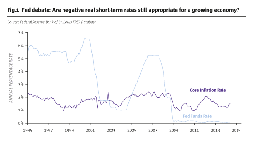
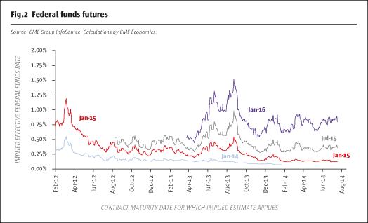
Delving deeper into the Brexit case study, we can hypothesise about the before and after probability distributions. Fig.1 shows the before picture — prior to the Brexit vote, there were two possible outcomes, with the British pound centered around $1.50/GBP if the outcome was “Remain”, and centred around $1.33/GBP if the vote was to “Leave.” As shown in Fig.2, when it became clear that the vote was to “Leave”, the market re-centred with a single-mode distribution around $1.33/GBP.

The actual second-by-second price movements on Friday, 24 June, 2016, as markets digested the referendum results were pretty exciting. There are some extremely critical observations and takeaways from the second-by-second unfolding of the price discovery process. Namely, 1) there was a distinct price break, in this case downwards, as the referendum results were reported, and 2) there was an upward shift in the volatility regime.

We focus on these two observations because they are central to options pricing. The basic Black-Scholes options pricing model, developed in the early 1970s, makes no less than 10 simplifying assumptions, such as no one pays taxes, unlimited borrowing at the risk-free interest rate, and more. For event risk lessons, however, the two assumptions that truly matter are the price continuity assumption and the constant volatility regime assumption. Price continuity means that economists, as they are wont to do, have assumed away the possibility of price jumps or breaks, such as seen on post-Brexit day. The constant volatility regime assumption means that an upward shift in volatility, such as experienced on post-Brexit day, was not supposed to happen. Professors Black and Scholes made these assumptions to simplify the options pricing model.  In the decades since the Black-Scholes model was first published, many scholars have relaxed these two assumptions, at great complications to the mathematics, however, showing that when price jumps and volatility shifts are possible, a basic Black-Scholes model may give highly inappropriate results.

The takeaway lesson here is to remember that when event risk is likely, price jumps render delta hedging strategies for options as ineffective, and the volatility shift likelihood means that actual volatility may exceed historical and implied volatilities (as calculated by the basic Black-Scholes pricing model).

Thus, when severe event risk is present, options can offer considerable advantages for risk management, specifically because options embed a view on volatility and allow one to cope with price jump risk in a way that directional hedging and other tactics such as delta hedging cannot do alone. Our conclusion is that options are one of the best vehicles for managing event risk – only, however, if one recognises the need for more advanced options pricing models that consider price jumps and volatility shifts are likely possibilities and do not assume they do not exist.

All examples in this report are hypothetical interpretations of situations and are used for explanation purposes only. The views in this report reflect solely those of the author and not necessarily those of CME Group or its affiliated institutions. This report and the information herein should not be considered investment advice or the results of actual market experience.