Most investors tend to believe that stocks are a good—perhaps even the best—investment in the long run. However, the reason for expecting good performance from stocks is perhaps not always clearly articulated: Quite simply, it is because they are risky.
For an investor in the US, US Government debt is generally viewed as being risk-free, if we ignore inflation risk. This investor would rank investment-grade senior corporate debt as slightly more risky than Treasury bonds (with AAArated debt viewed as less risky than AA, followed by A, and so on). Next in the hierarchy would come subordinated debt, preferred stock, and common stock would bring up the rear. The reason stocks are the riskiest investment is that they are at the bottom of the pecking order in terms of their claim on the company’s profit or cash flow. But the reason they can also be the most rewarding is that they are entitled to all residual profits, after paying off the other more senior claims in the corporate capital structure.
Generally, investments with higher risk are expected to yield higher returns as an incentive to investors. Here, we do not address the issue of return. We simply focus on the risk of various stock-bond portfolios, and examine how much of this risk comes from their components, and, in particular, from stocks.[1]
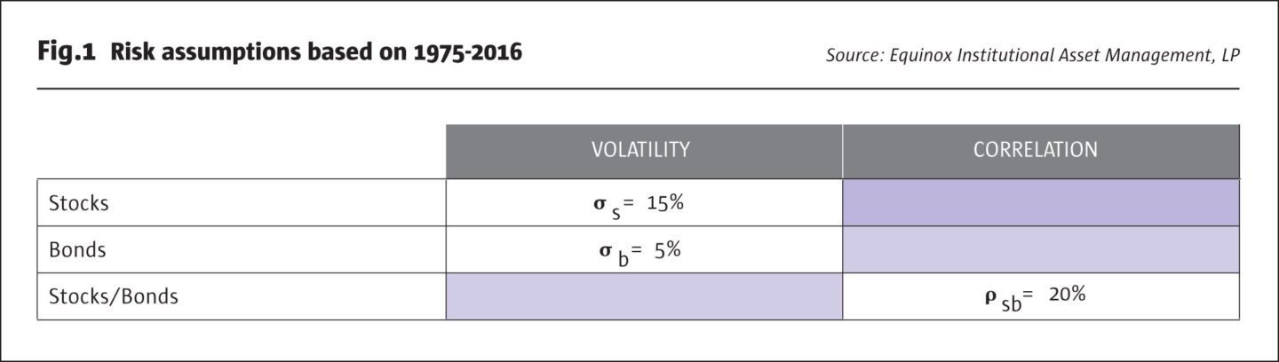
We do not know how volatile stocks and bonds will be in the future. We could use historical volatility as a projection, but the realized volatility of any asset depends on both the time period and the horizon over which it is measured. We therefore make some assumptions that are based on the realized values for the period 1975-2016 (the point we are trying to make here does not depend on the exact assumptions).
In Fig.1, we illustrate the assumed volatilities for stocks and bonds, and also the assumed correlation between them. We denote volatility with the Greek letter σ (sigma) and use subscripts ‘s’ and ‘b’ for stocks and bonds, respectively. The correlation is denoted by the Greek letter ρ (rho), with both ‘s’ and ‘b’ as subscripts, denoting that this is the correlation coefficient between stocks and bonds.
In order to analyze how much of the risk of a stock-bond portfolio comes from each of its components, we need to understand how the volatility of a portfolio is calculated. Fig.2 illustrates the formulas behind the calculations.
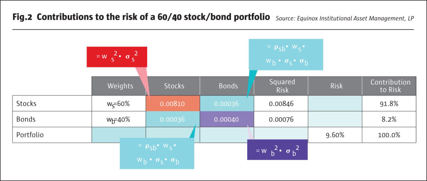
The risk of a stock-bond portfolio consists of four different pieces. For the sake of simplicity, we call them:
- the risk of stocks alone,
- the risk of bonds alone,
- the “co-risk” of stocks and bonds, and
- the “co-risk” of bonds and stocks.
The risk of stocks alone is given by the squared value of the allocation to stocks (60% in our example) multiplied by the squared valued of the risk of stocks (assumed to be 15%). This value turns out to be 0.00810.
The risk of bonds alone is given by the squared value of the allocation to bonds (40% in our example) multiplied by the squared valued of the risk of bonds (assumed to be 5%). This value is 0.00040.
The “co-risk” of stocks and bonds is given by the product of five quantities: the allocation to stocks, the allocation to bonds, the risk of stocks, the risk of bonds, and the correlation between stocks and bonds. This is equal to 0.00036. The “co-risk” of bonds and stocks, by symmetry, is also 0.00036.
Adding up these four numbers, we get 0.00922. The square root of this gives us 9.6%, the volatility of the 60/40 stock/ bond portfolio.[2]
What is the contribution of each component?
The risk of stocks alone plus the shared risk of stocks and bonds is 0.00846, which is 91.8% of the total squared risk, which is 0.00922. Thus, stocks contribute almost 92% of the portfolio’s risk, while bonds contribute the remaining 8.2%!
Upon reflection, perhaps this should not be a surprising result. The risk of stocks is three times as high as bonds (15% vs. 5%), and the allocation to stocks is 1.50 times the bond allocation (60% vs. 40%). These two factors combined result in the high contribution of stocks to portfolio risk. Many investors mistakenly believe that a 60/40 stock/bond portfolio is “well diversified” relative to an all-stock portfolio. In fact, even though this may appear true given that the portfolio’s risk is only about 64% of the risk of stocks (9.6% vs. 15%), the fact remains that 92% of this lower total risk still comes from stocks.
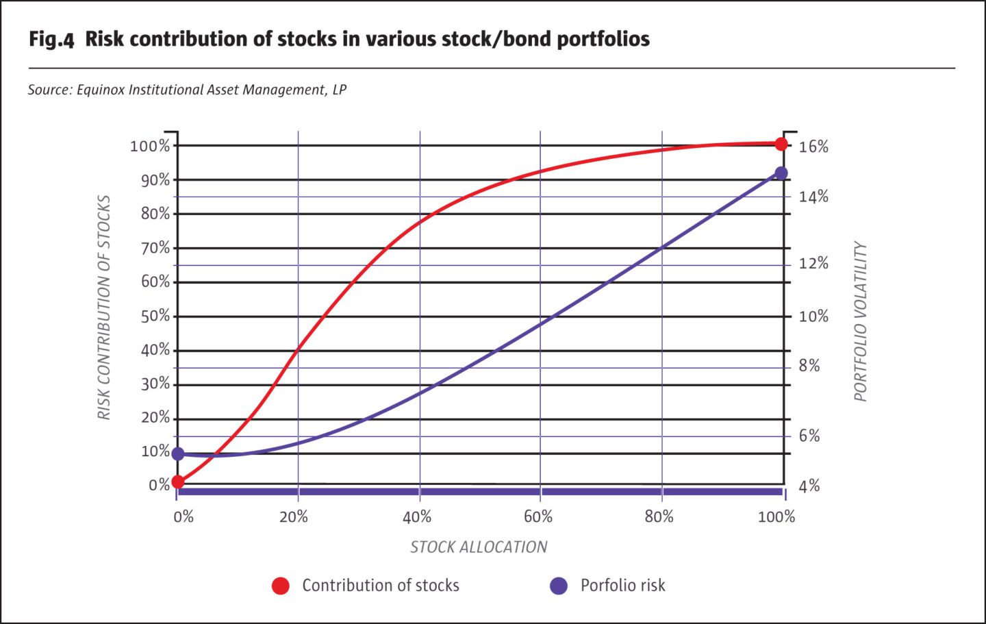
In going from an all-stock portfolio, where 100% of the risk comes from stocks, to a 60/40 portfolio, the risk contribution of stocks falls to about 92%. In Fig.3, we show the corresponding result for other portfolios, ranging from all-stock to all-bond. The results are also depicted graphically.
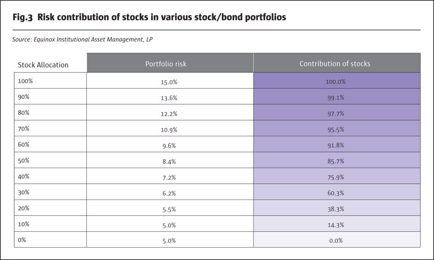
For an all-stock portfolio, all of its total risk of 15% (depicted on the right-hand vertical axis) comes from stocks. If we diversify into an 80/20 stock-bond portfolio, total risk falls to 12.2%, but almost 98% of this risk is still attributable to stocks. We have already seen the results for a 60/40 portfolio: almost 92% of portfolio risk comes from stocks. Even if we diversify further and consider a 40/60 portfolio, nearly 76% of its total risk, which is 7.2%, still comes from stocks. Even a portfolio with only 20% allocated to stocks derives almost 40% of its risk from them.
It bears repeating that risk is only one dimension, the other being return. While portfolio risk drops with the allocation to stocks, so does the expected return of the portfolio. In the long run, stocks must be expected to earn higher returns than bonds, in order to compensate investors for their higher risk. Investors, in conjunction with their advisors, need to decide the level of total portfolio risk with which they are comfortable.
This will likely be a function of several variables, including age and position in the life-cycle, wealth, liquidity, and attitude towards risk.
In part two, we address the topic of extended diversification: How does investing in other non-correlated asset classes affect total portfolio risk and its components. This may be a particularly important issue at a time when global stock markets are near all-time highs while volatility appears to be almost unusually low.
Part Two
In the first part of this Insight, we focused on the risk of various stock-bond portfolios and examined how much of this risk comes from their components.[3] Based on some reasonable assumptions about the volatility of stocks and bonds, and the correlation between them, we showed that most of the risk comes from stocks.
For an 80/20 stock-bond portfolio, 98% of total risk is attributable to stocks, and for a 60/40 portfolio, the contribution is as high as 92%. If we diversify further away from stocks, and consider a 40/60 portfolio, 76% of its total risk still comes from stocks. Even a portfolio with as little as 20% allocated to stocks derives almost 40% of its risk from them.[4] An implication of these findings is that equity markets will have a big impact on realized portfolio returns. While this can be beneficial during bull markets, it can result in crippling losses during market meltdowns such as 2007−08. And yet investors continue to hold significant positions in stocks, reaching for higher long-term returns while wrestling with shorter-term volatility.
In this Insight, we address the topic of diversification beyond bonds and into “alternative investments:” How does investing in other non-correlated asset classes affect total portfolio risk and its components? As an example of a non-correlated asset class, we pick managed futures.[5] Not knowing how volatile stocks, bonds, and managed futures may be in the future, we make some assumptions, as before, that are based roughly on the values realized during the period 1987-2016.[6]
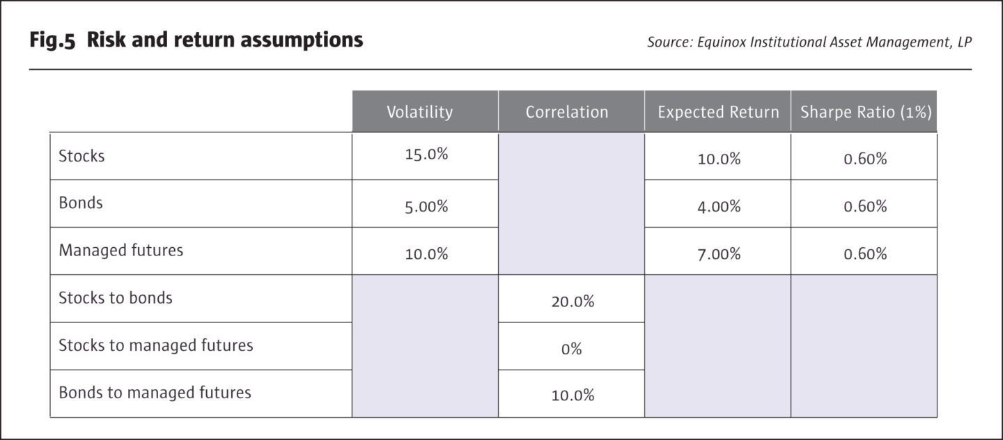
In Fig.5, we show the volatilities we assume for stocks, bonds, and managed futures, as well as the assumed correlations between each pair of asset classes. We also make what we believe are some reasonable assumptions about the expected returns on each asset class for the long run: We assume that the risk-free rate of interest will be 1%, and that all three asset classes will have the same Sharpe Ratio going forward.[7]
In Fig.6, we show the risk of hypothetical portfolios with a range of allocations to stocks and bonds, with the balance allocated to managed futures, so that the three allocations add up to 100%. Note that the portfolios at the three corners of the triangular array represent portfolios with 100% allocated to a single asset class out of the three (highlighted in yellow). Portfolios along the edges of the triangle represent two-asset portfolios: green are stock/ bond portfolio, pink are stock/managed futures, and blue are bond/managed futures.[8] Thus, a 50/50 stock/bond portfolio has a risk of 8.4%, a 50/50 stock/managed futures portfolio a risk of 9.0%, and a 50/50 bond/managed futures portfolio a risk of 5.8%. Note that these risks are in each case lower than the simple average of the two individual risks: this is the “free lunch” of diversification.
As a rule of thumb, the lower the correlation between two asset classes, all else equal, the relatively greater the diversification benefit.
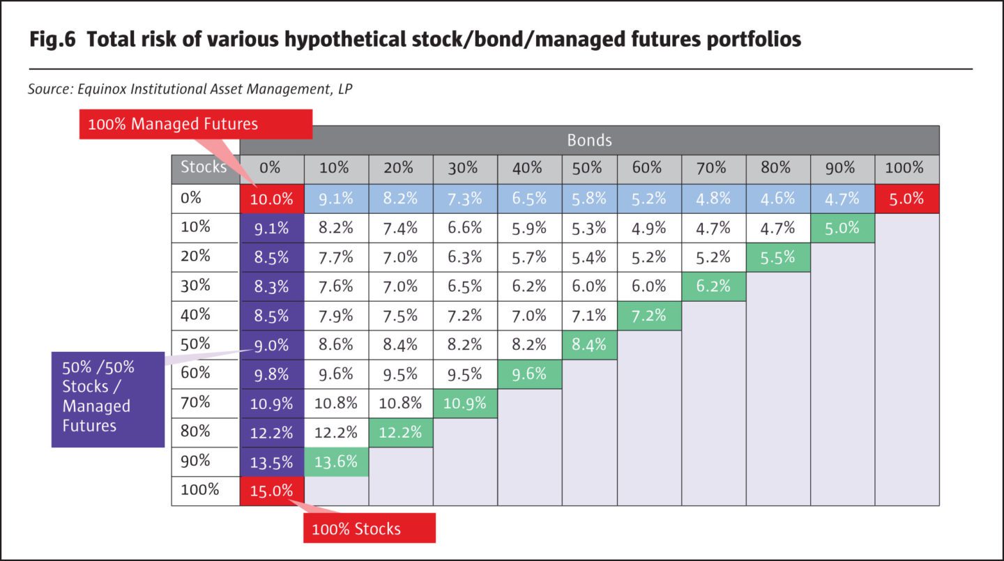
The 50/50 stock/bond portfolio’s risk is 8.4% compared to the average risk of stocks and bonds, which is 10% (the average of 5% and 15%); this represents a 16% reduction in risk. The correlation of stocks and bonds is assumed to be 20% in Fig.5. Stocks and managed futures are assumed to have a correlation of zero. The risk of the 50/50 stocks/ managed futures portfolio is 9%, which is 28% lower than their average risk, which is 12.5% (the average of 10% and 15%). This larger reduction in risk, 28% vs. 16%, is a consequence of the lower correlation of 0% vs 20%.
How would an investor decide which of these portfolios he/ she prefers? Should it be the portfolio with the lowest risk? That turns out to be the 80/20 bonds/managed futures portfolio, with a risk of 4.6%. However, this is mainly a consequence of the fact that bonds are generally the least risky of the three asset classes. We should also expect this low-risk portfolio to have a fairly low—perhaps the lowest—expected return, possibly too low for an investor who is more aggressive. As we have said before, looking at just portfolio risk without considering return—or looking at return without considering risk—only tells half the story. Investors, in conjunction with their advisors, need to decide the level of total portfolio risk with which they are comfortable. This will likely be a function of several variables, including age, life-cycle status, wealth, liquidity needs, and attitude towards risk.
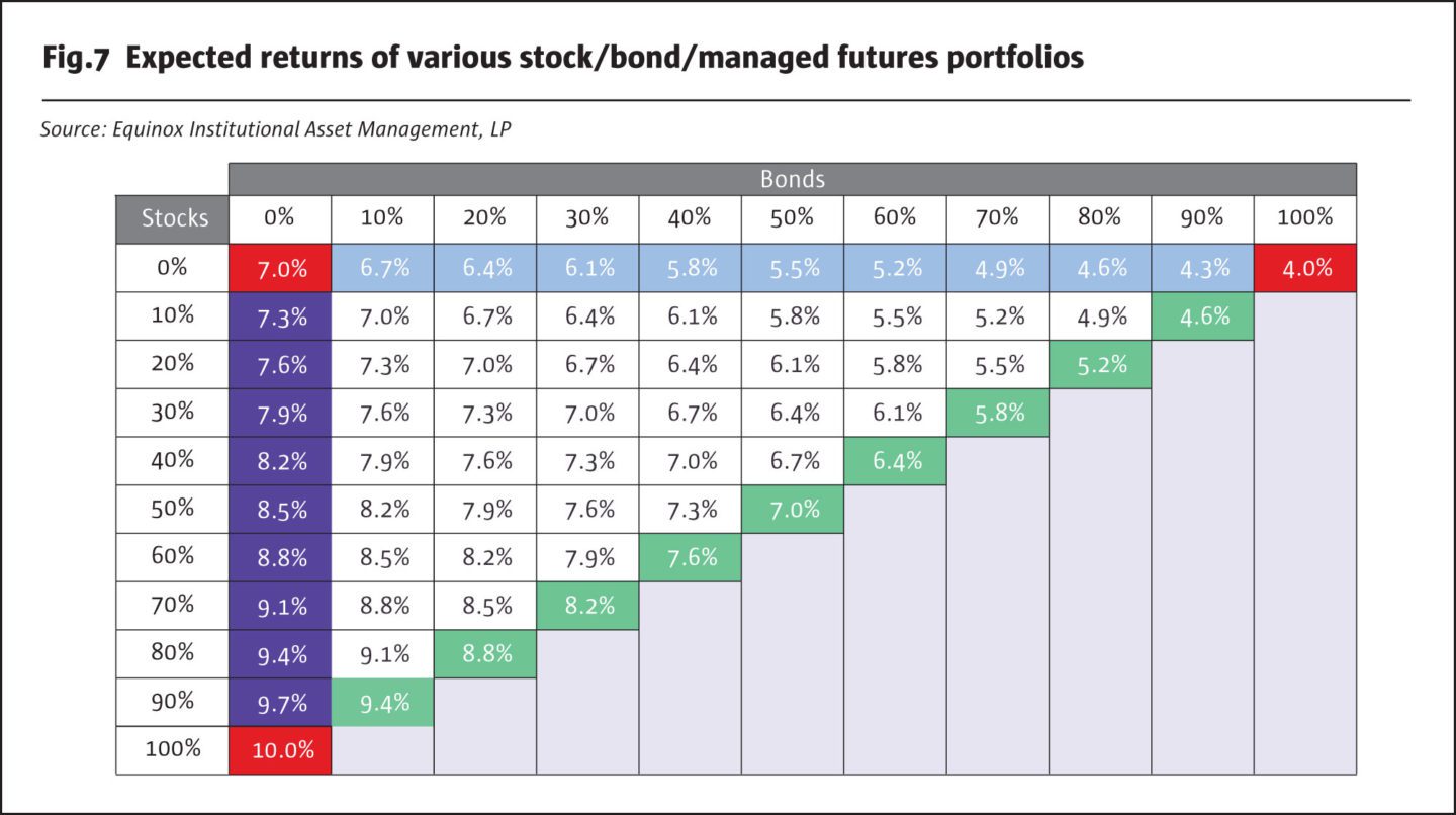
Let us now turn to the expected returns (based on our assumptions from Fig.5) of these portfolios, which are shown in Fig.7. As expected, portfolios with higher stock allocations tend to have higher returns, while those with higher bond allocations tend to have lower returns. Note that the expected return of any 50/50 portfolio is simply the average of the returns for its component asset classes; there is no “diversification” advantage (or disadvantage) for portfolio expected return as there is for portfolio risk.
One way to combine the information in Fig.6 and Fig.7 in an effort to seek out an “optimal” portfolio is to calculate the Sharpe Ratio for each portfolio. This ratio is simply a measure of how much “risk premium” a portfolio earns per unit of risk that it takes. To keep things simple, we assume a risk-free rate of 1%, and calculate the Sharpe Ratio for each portfolio:
Sharpe Ratio = (Portfolio Expected Return – 1%) / Portfolio Risk
For example, the 50/50 stock/bond portfolio has a Sharpe Ratio equal to 7% minus 1%, which is 6%, divided by its risk of 8.4%, which gives 0.72. All else equal, a higher Sharpe Ratio implies a more desirable portfolio.
In Fig.8, we show the Sharpe Ratios for the various portfolios. The “corner” portfolios, with 100% in a single asset class, all have the same Sharpe Ratio of 0.60, which was our assumption in Fig.5. The portfolio with the highest Sharpe Ratio, 0.95, turns out to be the 20/50/30 stock/bond/managed futures portfolio. Individually, this portfolio has an expected return of 6.1%, which is not highest. Nor is its volatility of 5.4% the lowest among all portfolios. It does have the highest reward-to-risk ratio, however, and is therefore in some sense the “optimal” or best portfolio in terms of the trade-off between risk and return.
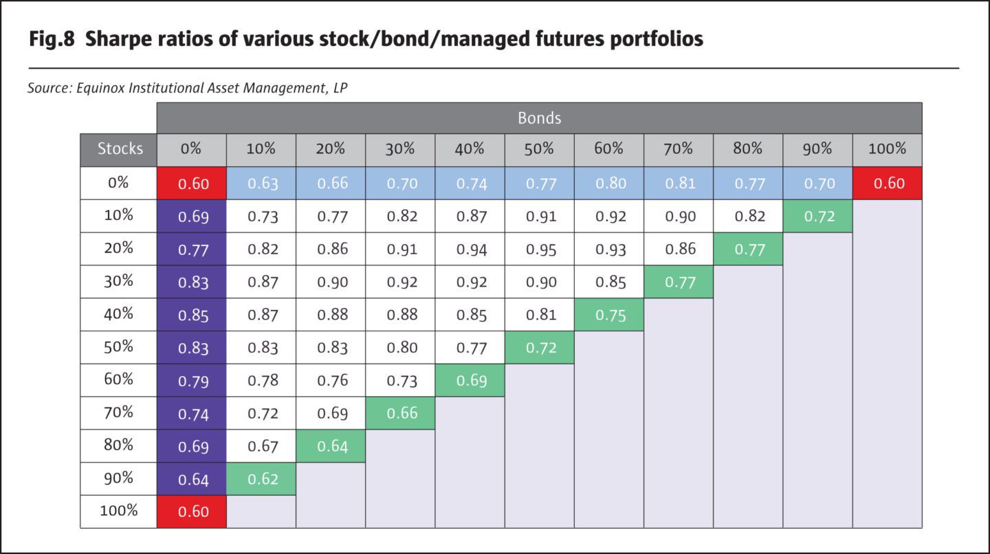
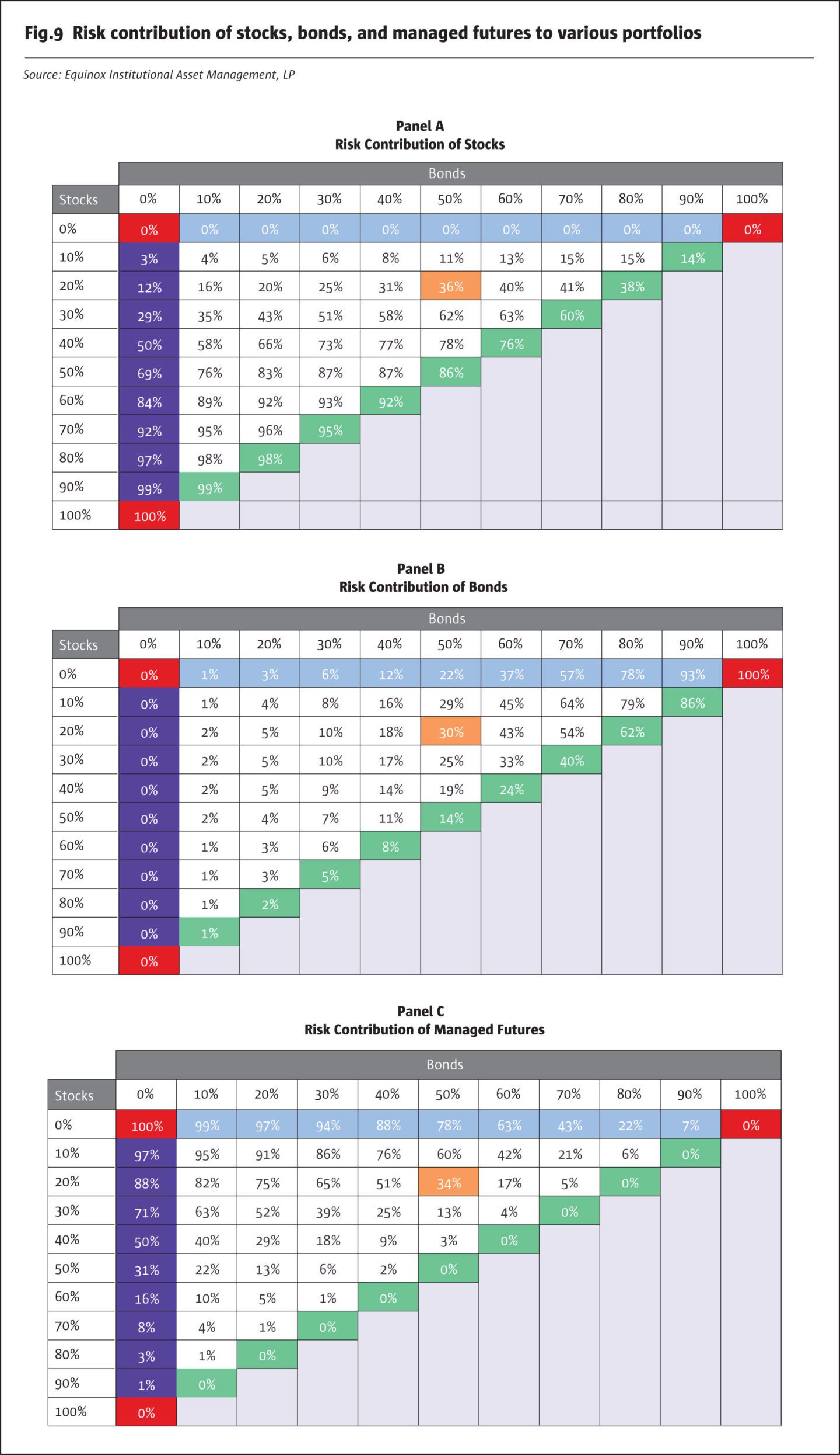
Consider the 20/50/30 portfolio from Fig.8, which had the highest Sharpe Ratio. It turns out that the three asset classes contribute almost equally to the risk of this portfolio: stocks contribute 36%, bonds 30% and managed futures 34%. A portfolio in which the risk contributions of various components are equalized is sometimes called a “risk parity” portfolio.[9] This turns out to be a very rough rule-of-thumb: it is not always necessary that the portfolio with the highest Sharpe Ratio is the “risk parity” portfolio, which is a term used to define the portfolio in which all the individual components contribute equally toward the total risk.
Using some very simple assumptions, we have shown that a “more diversified” portfolio, whose risk contributions are spread out across its component asset classes, turns out to have a higher reward-to-risk ratio than one with a significantly higher risk contribution from one asset class such as stocks. This reiterates one of the teachings of Modern Portfolio Theory (MPT): Diversification helps.
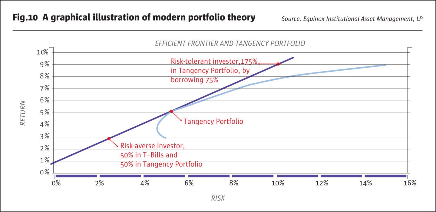
MPT goes on to state that the portfolio with the highest Sharpe Ratio, also called the “tangency portfolio,” is the optimal risky portfolio for all investors. Each investor has the ability to combine this portfolio (which turns out in equilibrium to be the “market portfolio”) with risk-free lending or borrowing, so that he/she ends up holding an overall portfolio still with the highest Sharpe Ratio, but with an appropriate level of risk. Relatively risk-averse investors combine the market portfolio with risk-free lending (i.e., investing in cash or T-Bills) to “dilute” their risk and earn a lower return. As shown above, a risk-averse investor can invest 50% of her total wealth in T-Bills earning 1% and 50% in the tangency portfolio, thereby reducing risk to about 2.7% with an expected return of about 3%. A more risk-tolerant investor can, in theory, borrow say 75% at the risk-free rate and leverage the risky portfolio to 175%, taking on greater risk of about 9.5% while seeking to earn a higher return of close to 9%.[10]
One constraint that MPT imposes on the tangency portfolio is that the allocations sum up to 100%, even when borrowing or lending is involved. In the next part of this series of Insights, we will examine the effects of relaxing this constraint: for example, we will examine portfolios with 50% allocated to managed futures, but in a 60/40/50 portfolio rather than a traditional 30/20/50 portfolio. Note that the allocations in the traditional portfolio add up to 100%, while those in the other portfolio add up to 150%.
We call this idea “extended diversification” or the “Power of &.”
Extended diversification may enable investors to potentially harness the combined benefit of their current portfolio AND managed futures. The traditional “OR” decision involves selling part of the existing stock and/or bond holdings in order to gain exposure to a diversifying asset class such as managed futures: the portion that is allocated involves a choice between managed futures OR stocks/bonds. Thus, the allocation to managed futures may incur the opportunity cost of forgoing the returns that stocks and bonds might have continued to earn.
Extended diversification seeks to allow investors to hold on to their stocks and bonds AND allocate to managed futures, without the opportunity cost of selling stocks and bonds.
In many cases, by managing allocations appropriately, this can potentially be achieved without taking on the significant increase in risk of a portfolio that is leveraged traditionally through borrowing.[11]
Footnotes
- Here, we use the standard deviation of returns, also called volatility, as the measure of risk. For most traditional assets, and when dealing with returns measured over reasonably long horizons, volatility serves as an adequate proxy for risk.
- Note that this is lower than the weighted average of the volatilities, which is 60% of 15% plus 40% of 5%, i.e., 11%. The fact that the portfolio volatility is only 9.6% rather than 11% represents the benefit of diversification: the correlation coefficient is only 20%, and this results in lower risk. If stocks and bonds were perfectly (100%) correlated, the portfolio’s volatility would have been 11%.
- The Risk Contribution of Stocks, Insight, May 2017. We use the standard deviation of returns, also called volatility, as a measure of risk. For most traditional assets, and when dealing with returns measured over reasonably long horizons, volatility serves as an adequate proxy for risk.
- These results are repeated in Panel A of Table 5.
- We have discussed elsewhere the benefits of diversification in general, and diversification through managed futures in particular: see, for example, our Insights, Harnessing the Potential Benefits of Managed Futures (2016), Speaking of Correlation (2017), and Allocating to “Liquid Alternatives” – The Importance of Correlation (2016).
- For the sake of consistency, we use the same values for stocks and bonds that we used in our previous Insight.
- We discuss Sharpe Ratio later in the paper. This assumption of equal Sharpe Ratios has the effect of seeking to minimize the bias in favor of any asset class. The expected returns we assume are loosely based on their historical realized values. The substantive conclusions of this Insight do not depend on the assumptions, however.
- The green-shaded numbers are identical to those shown in our previous Insight
- Since there can be different measures of risk, there is no unique definition of risk parity.
- Of course, these prescriptions are based on a number of simplifying assumptions, many of which are not necessarily reflective of financial markets in practice.
- This may be possible for an asset class such as managed futures, where only a small amount of margin or collateral needs to be posted in order to gain exposure. Extended diversification may afford investors the opportunity to post their existing stocks and bonds as collateral rather than having to sell them.
About the author
Dr. Ajay Dravid has over 30 years of experience in industry, academia, and financial services. He has published numerous papers in leading academic and practitioner journals including Journal of Finance, Journal of Financial Economics, and Journal of Derivatives. Dr. Dravid received a BSc in Physics from the University of Poona (India), an MA in Physics from SUNY at Stony Brook, an MBA in Finance and Marketing from the University of Rochester, and a PhD in Finance from the Graduate School of Business at Stanford University.
- Explore Categories
- Commentary
- Event
- Manager Writes
- Opinion
- Profile
- Research
- Sponsored Statement
- Technical
Commentary
Issue 131
The Risk Contribution of Stocks
Parts one & two
Ampersand Portfolio Solutions
Originally published in the April 2018 issue