One issue faced by fund managers is developing expectations for the future returns of their products. This task for CTAs is made more complicated by the fact that many strategies are designed to be uncorrelated to conventional market indices, benchmarks and indicators. An approach to generating such a forecast is to relate strategy returns to bespoke factors that pertain to the known characteristics of the strategy (e.g., trend following or mean reversion). If some of these factors can themselves be predicted with accuracy, then in principal that prediction can be extrapolated to the returns of the strategy.

While CTA returns tend to be uncorrelated to commonly used factors (such as Fama-French factors), it is possible to follow this approach and define custom indicators that have explanatory value. An example of this is a market trend index: if markets exhibit strong, persisting trends, one would expect trend following CTAs to perform well. If trends are weak or nonexistent, trend following CTAs ought to have flat or negative performance. This effect can be measured quantitatively.

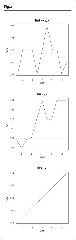
There are many ways to define the concept of “trend.” A market trend index is one possible approach, which happens to be a useful explanatory factor for CTA (as defined by the Newedge CTA index) performance. The first step in computing the market trend index is to calculate a signal to noise ratio (SNR) for asset prices over a given lookback period. The SNR is simply the absolute price change over the lookback period divided by the sum of the absolute daily price changes. The lookback period may vary depending on the length of trends of interest, but two months or longer tends to relate sufficiently closely to CTA returns in terms of linear correlation to a benchmark index. The closer the price path is to a straight line, the higher the SNR. A perfectly straight line will have an SNR of 1, while a completely flat path will have an SNR of 0. In Fig.1 are some examples with generated data.

In the second step tocomputing the market trend index, the SNR for individual futures is aggregated into an index by taking the relevant average. For example, the equity sector trend index is the average of the SNR for equity futures such as the Dow Jones Industrial Average, S&P 500 E-Mini, Eurex DAX 30 and the FTSE 100. An overall trend index would be the average among all tradable markets.

Because this market trend index is a measure of how “trendy” futures prices are, we expect it to correlate with CTA trend follower performance over comparable time frames. In Fig.2 is a plot of the Newedge CTA index quarterly returns (blue) alongside the SNR trend index (red) computed for the same period.

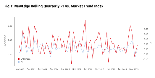
The correlation between these two series is 62%. Fig.3 the same data are depicted in scatterplot form.

 
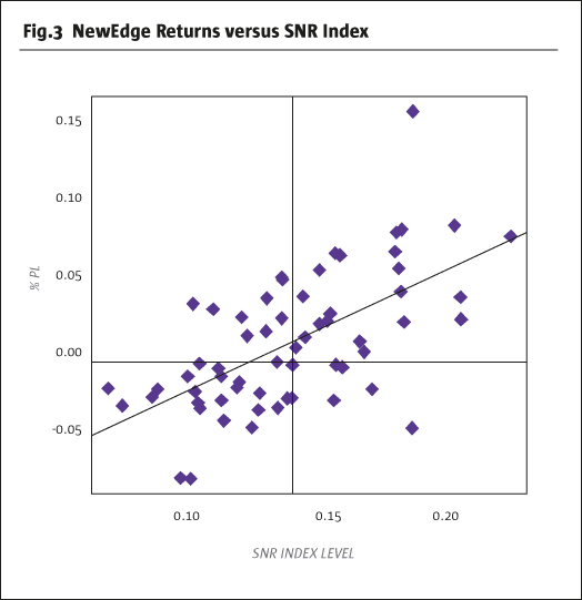
Notice the clustering of points around the regression line.

Given this quantitative definition of the level of trend, statistical tests can be performed to examine whether there are consistent patterns in the level of trend.

One question we hope to address using the SNR is how fourth quarter trends compare to the remainder of the year, on both a sector and overall level for futures. We can start by examining the SNR of a representative set of futures contracts from four different sectors (equity indices, commodities, currencies, and interest rates) from 1990 onwards. The average SNR from Q4 can be compared to the average SNR from quarters 1-3 by using a paired Student’s T-test. The null hypothesis of Q4 SNR equaling Q1-3 SNR is rejected in favor of the alternative that Q4 SNR is greater at the 10% level (p-value = 0.090, t=1.37). While this level of significance may only be modest, it does suggest that, at the very least, the trendiness of all quarters is not necessarily uniform.

To take this analysis a step further, we form sector-level SNR indices, which are the individual futures’ SNR indices averaged at the sector level. Since there are only 4 sectors we compare the values of Q4 SNR to the values of Q1-Q3 SNR. This results in an unequal sample size (25 observations for Q4 PL, 75 for Q1-Q3 PL), necessitating a Welch Two Sample T-test. However, this test has the unfortunate consequence of assuming that each sample follows a Gaussian distribution, but quarterly SNR fails a Jarque-Bera test for normality. Regardless, the t-test in Table 1 might give some insight into the source of the differing Q4 SNR.

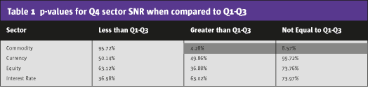
Referring to Table 1 of p-values, we find that only one sector deviates at the 10% level in Q4 from the remainder of the year. Commodities tended to have stronger trends in Q4.

If this Q4 effect on trends exists, and if CTA returns relate positively to the trend index, we should also expect to see higher than average CTA returns in Q4. We can perform the same t-test on Newedge CTA index quarterly returns. The null hypothesis that Newedge CTA Q4 returns have the same mean as Q1-Q3 is rejected in favor of the alternative that Q4 is greater at the 1% level (p-value = 0.00135, t=3.17). The average annualised return in Q4 was 14.4% vs. 2.67% in the remaining quarters. This effect is also apparent in other CTA indices, namely the Newedge CTA Trend Index, which has an even starker difference at 22.7% annualised in Q4 vs. 2.6% in the remaining quarters.

The available evidence suggests that commodity trends tend to be much stronger in Q4, possibly leading CTAs to perform much better than average during this period. In future research it may be worthwhile investigating what contributes to these Q4 trends (perhaps relatively low volatility or seasonal effects reflected in prices), as well as how to incorporate this information in the systems underlying a CTA strategy.

Relating SNR to CTA Crisis Alpha
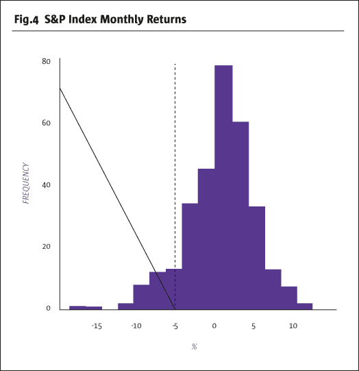
One appealing characteristic of CTAs is their performance under periods of market distress, or crisis. If we flag periods as crises using the following criterion: S&P 500 Index monthly returns below their 10% quantile (-4.7%), we observe that the Newedge CTA index realised an annual return of 19.5% in these months, compared to 3.3% in non-crisis periods. Based on the previous analysis, it is possible that this crisis alpha is in part driven by an increase in the level of trend in markets (e.g., downward trend in the case of the equity markets). If CTAs can exploit the persistence of such trends in a crisis, they stand to benefit from prolonged downturns.

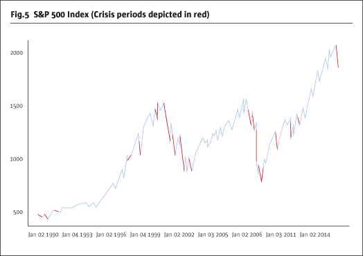
Returning to the S&P 500, we may be able to gain insight into the source of crisis alpha by examining how the aggregate level of trend, measured by average SNR, changes during crises. Applying a Welch Two Sample T-test comparing crisis aggregate SNR values to observations from the rest of the sample (1990 onwards), we find that we may reject the null hypothesis that the two samples have equal mean in favor of the alternative that crisis SNR is greater at the 5% significance level (p-value = 0.042, t=1.79).

We may apply the same test at the sector level to see if a subset of futures markets are trendier during these periods. See Table 2.

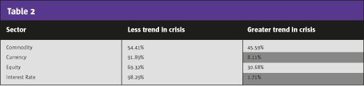
Contrary to the assumption that successfully exploited equity market trends are the source of crisis alpha from CTAs, equity trends as measured by SNR do not appear to differ at the 10% significance level.

However, interest rate trends, and to a lesser extent currency trends, deviate from their non-crisis levels. This may be because equity downturns are preceded by persisting trends in these other sectors that are followed accurately. While the understanding of the source of CTAs’ crisis alpha remains incomplete, SNR provides some insight into market behavior during these events.

Conclusion
Fourth quarter historically has been more favorable for trend following managed futures programs in comparison to the first 3 quarters.  Commodities appear to have the strongest trends in the fourth quarter.

In periods of stress in the stock markets the trend followers have provided crisis alpha.  The trendiness as defined by signal to noise ratio in these conditions appears to be strongest in interest rates and currencies.