Introduction
The turbulence of 2018 made it a difficult year for most systematic investment products. To the surprise of several investors, many of these quant products had been sold as market neutral. In particular, the new breed of alternative risk-premia (ARP) products – that had flooded the market a few years prior to 2018 – performed exceptionally badly. For example, the composite HFR Bank Systematic Risk-premia Multi-Asset Index lost -18%, in comparison with a loss of -4% on the S&P 500 total return index. However, traditional alternative asset classes also underperformed, with the flagship HFRX Global Hedge Fund Index losing -7% and the SG Trend Index losing -8%.
In the face of such losses, both investors and managers are asking how and why so many quant strategies underperformed? Still more importantly, what are the implications for the diversification of traditional equity-bond portfolios and alternative investments? In particular, since trend-following CTAs belong to a handful of tried-and-tested diversifiers, why did trend-followers not diversify in 2018?
To address such questions, we first intend to look at how trend-following programs are expected to perform when crises last for extended periods of at least two months, because trend-followers need to adjust to profit from sustained crises in equity markets. Second, we shall focus on the way in which the risk profile of ARP products, hedge funds, and trend-following CTAs can change in bear and bull market regimes because of their potential exposures to tail-risk. We analyse the risk-premia alpha in these products by taking into account regime-conditional risk.
For this analysis, we are proposing a new quantitative model to explain the risk of investment strategies by accounting for extreme market conditions and for their exposure to tail risk, such as selling volatility and credit protection. We apply this model to the cross-sectional risk attribution of about 200 composite indices of hedge funds and ARP products. We show that there is a strong linear relationship between risk-premia alpha and the tail risk of systematic ARP strategies. We can demonstrate that our model explains nearly 90% of the risk-premia for volatility strategies and about 35% of the risk-premia for hedge fund and ARP products. In this way, most ARP and hedge fund type products can be seen as risk-seeking strategies. Importantly, our model predicts that ARP products offer smaller risk-premia compensation compared to hedge funds.
We are able to illustrate that, interestingly, trend-following CTAs are exceptions since they belong to defensive strategies with negative market betas in bear regimes, yet risk-premia alphas for CTAs are insignificant. CTAs cannot be seen either as ARP products with positive risk-premia alpha from exposures to tail risk, or as defensive products with negative risk-premia designed to reduce tail risk, such as long volatility strategies. Instead, trend-following CTAs should be viewed as an actively managed defensive strategy with the goal to deliver protective negative market betas in strongly downside markets along with risk-seeking positive market betas in strongly upside markets. Overall, after adjusting for the downside and upside betas, the risk-premia alpha of CTAs is insignificant. Yet, because of the negative protective betas in bear markets, trend-followers well deserve their place as diversifiers in alternative portfolios to improve risk-adjusted performance and capture risk-premia alpha on a portfolio level, as we will show in the last section.
Finally, since our risk-attribution model assumes conditional equity betas in specific market regimes, we are able to illustrate the misunderstanding behind strategies claiming to be “zero-correlated” and “market-neutral”. Given a specific market regime, most typically in the bear regime, many risk-premia strategies tend to produce a strong exposure to equity markets because of their hidden tail exposures. For example, a strategy selling delta-hedged put options would have a small market beta during normal regime; yet the strategy would exhibit a significant market beta during crisis periods because of its negative gamma and vega exposures. When we analyse systematic strategies unconditional to market regimes, the performance may appear to be smooth and uncorrelated because of the aggregation across different regimes.
We will conclude the introductory section and our article by answering the above questions in the following way. Firstly, ARP strategies are expected to perform well during normal regimes. However, since the excess performance of these strategies is derived from a hidden tail risk, these strategies are expected to underperform during turbulent markets, as in 2018. To earn risk-adjusted alpha from these products, investors need to look at long time horizons that include both bull and bear markets. Second, while the performance of trend-following CTAs is not derived from risk-premia alpha as compensation for hidden tail risks, the performance of trend-followers is conditional on trends lasting for sustained periods. Since trends reversed rapidly multiple times during 2018, trend-followers underperformed. As a result, in what proved to be an extraordinary year, both ARP products and trend-followers underperformed, but for different reasons.
Going forward, investors and allocators need to understand how different strategies are expected to perform during bear and normal markets and how to diversify their portfolios accordingly. Our results provide a valuable aid in quantifying the hidden tail behaviour of systematic strategies as well as suggesting an approach for the risk attribution and diversification of alternative portfolios.
How trend-following works
Trend-following is an active strategy that seeks to leverage both sustained downside and upside trends in the markets. Nevertheless, a common question from the investment community is why trend-following programs can be too slow to benefit from quick and steep reversals in broad markets. How, for instance, can we explain the poor performance of the SG Trend index in 2018?
This section focuses on illustrating how trend-followers rely both on the duration of trends and on how they can deliver protection during extended equity market crises. For our illustrations, we turn to the actual performance of the SG Trend Index, which serves as a benchmark in the trend-following industry, and the S&P 500 Total Return Index as the proxy for the equity index.
Typical trend-following CTAs trade in a variety of liquid futures markets covering major global stock indices, fixed-income instruments, short rates contracts, FX and commodities. Trend-followers can take both long and short positions with leverage controlled through targeting of portfolio risk or volatility. The objective of trend-following CTAs is to identify medium to long-term trends in a systematic way. The implementation of a trend-following strategy on an instrument level includes two key elements: signal generation and sizing of exposure. Finally, implementation at a portfolio level involves sophisticated risk-based allocation and efficient trade execution.
Simplified trend-following strategy for illustration
To create a hypothetical performance of a trend-follower in action, we applied a simplified trend-following strategy to the S&P 500 index during the first three months of the global financial crisis, from September 2008 to November 2008. This simplified strategy became representative of a trend-following approach in the real world.
We began with the assumption that we had launched our strategy on the last day of August 2008 with zero exposure to the equity index. Then, at the end of each trading day, we computed the cumulative return of the equity index and the trailing minimum of the cumulative return. The equity exposure of our simplified trend-following strategy at the end of each day was set to the trailing minimum observed the day before. The rationale behind sizing our exposure was straightforward. We had established that the equity index was on the downside trend (signal part), but we were not certain about the potential extent of the correction (exposure part). As a result, we increased our short position gradually and set the exposure to the running minimum of the cumulative return from the launch. Since the running minimum changes slower than the cumulative return, we avoided over-trading in case the equity index experienced a bear market rally.
The bottom of Figure 1 illustrates the cumulative return of the equity index and the equity exposure of our simplified trend-following strategy. In the top part, we show the P&L of the strategy and its trend-line which grows in a quadratic way. In Figure 2, we plot trailing weekly returns of the trend-following strategy against trailing weekly returns of the equity index during each of the three months.
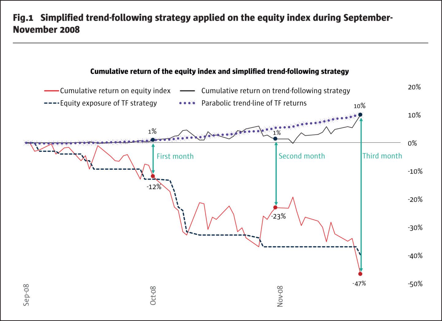
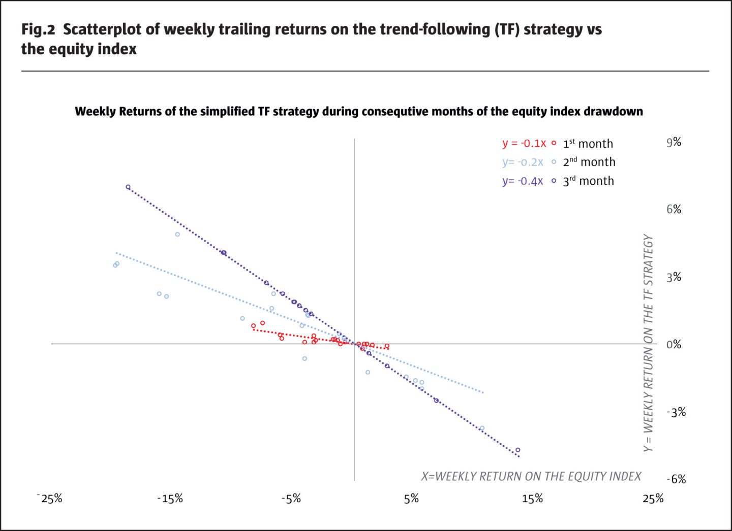
Within the model, as the equity crisis unfolds, the performance of our simplified strategy changes in the following manner. During the first month of the crisis, the equity exposure of the trend-following strategy is too small to capitalise on the downside trend. The strategy has a very small negative beta of -0.1 to the equity index and generates a return of only +1%, while the equity index declines by -12%.
In the second month, the trend-following strategy starts to plug into the bearish trend by achieving stronger beta of -0.2 yet generating only about +1% since the inception of the crisis despite the equity index losing -23%.
Finally, in the third month of the crisis, following sustained underperformance of the equity index, the trend-following strategy establishes a large short exposure. Accordingly, the strategy beta decreases to -0.4 while the total crisis performance reaches +10% against the loss of -47% on the equity index.
Our illustration highlights the most important aspect of trend-followers’ performance: the exposure of a trend-following program changes in a non-linear way though the course of equity correction. The trend-following program might not capture the initial stages of a new trend, but the program would still benefit from the further stages of the trend should it persist.
Trend-followers can deliver crisis beta
As we have illustrated, the performance of trend-followers is difficult to predict at the start of equity drawdowns because they may have sizable long exposures to the equity index. In 2018, we witnessed this effect twice, in February and in October. Prior to both corrections, trend-followers amassed sizeable long equity exposures after an extended equity rally. Consequently, they experienced steep losses when the equity index corrected sharply.
In Figure 3, we provide further illustration of the relationship between the duration of the equity drawdown and the performance of the SG Trend Index. It appears as follows:
1. The red bar shows the performances of the S&P 500 Index during the first month of the equity correction lasting more than a month and triggered when the monthly return is less than -4%.
2. The red line measures the drawdown of the S&P 500 Index from peak to trough.
3. The purple bar is the net performance of the SG Trend Index during the first month of the equity correction. The green line is the performance of the SG Trend Index during the entire period of the equity correction from peak to trough.
4. The purple and red columns show the marginal performance after the first month of the correction to the bottom of the drawdown.
5. The labels at the bottom of the chart show the total duration of the equity drawdowns.
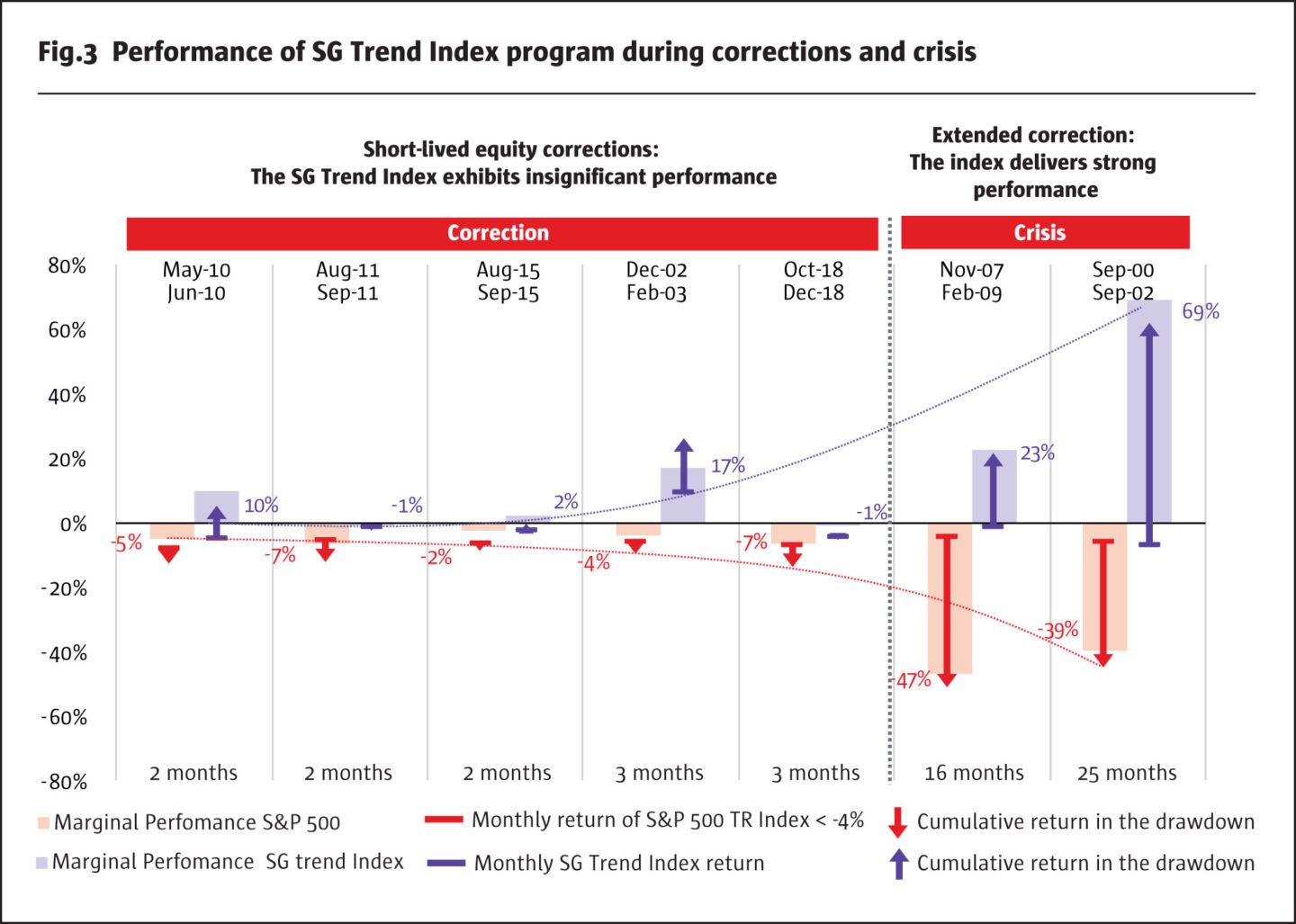
For example, in November 2007, when the last bear market started, the equity index fell by -4% in the first month and the equity drawdown continued until February 2009 with a total loss of -51%. During the same period, the SG Trend Index lost -1% in the first month but gained +22% over the entire period delivering crisis beta. More recently, in October 2018, the equity index corrected by -7% and the drawdown is still ongoing (as of end of December 2018) with a total loss of -14% from the last high watermark. During the same period, the SG Trend Index lost -4% in October and was not yet able to capitalise on new trends with the index losing -5% since October. To summarise, the essence of trend-following is to benefit from sustained trends lasting from a few weeks to a few quarters.
Performance in bear and bull markets across asset classes
So far, we have compared the performance of the SG Trend Index against the equity index. Do trend-following CTAs perform equally well when other major asset classes are in bear or bull regimes?
For the following illustration we have applied our conditional regression model – to be formally introduced in the next section – to identify bear and bull regimes for four major asset classes. Table 1 introduces the asset classes and corresponding position that a trend-following program would take in this class to benefit from either a bear or a bull regime. For better visualisation in Figure 4, we have multiplied the performance of positions in long and short bonds and long and short USD dollar by -1 to align them with the corresponding performance of positions in short and long S&P 500 index and commodities.
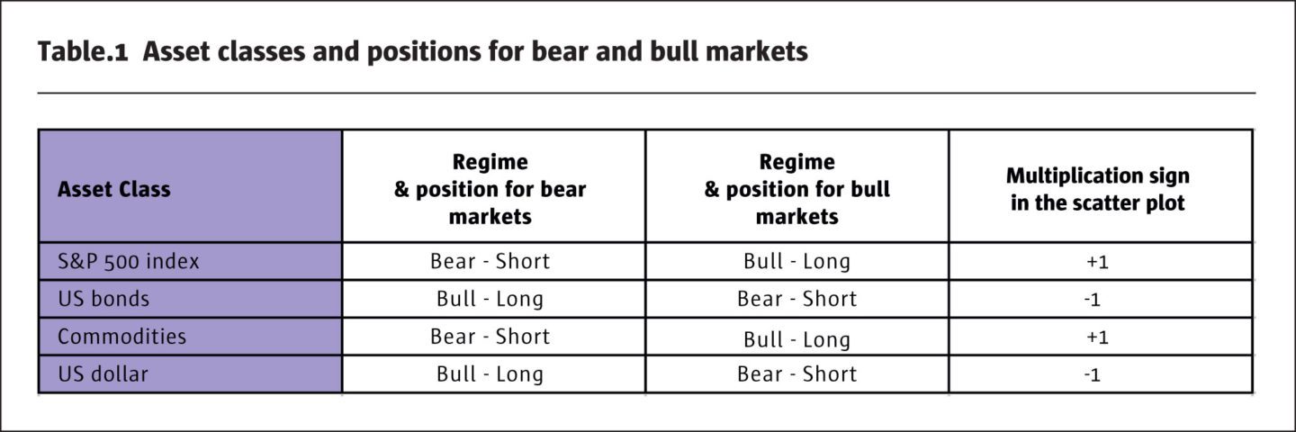
The left part of Figure 4 displays the scatter plot with the performance of asset classes in bear markets and the corresponding performance of the SG Trend index. The size of bubbles is proportional to the number of simultaneous crises across asset classes. The regression equation is the beta attribution of the asset class to the performance of the SG Trend index. For example, for a short position in the S&P 500 index, a loss of -10% is expected to contribute +5.4% to the SG Trend index. The right part of Figure 4 shows corresponding performances in bull markets. Here, a gain of +10% on the S&P would contribute a gain of 1.5% in the SG Trend Index.
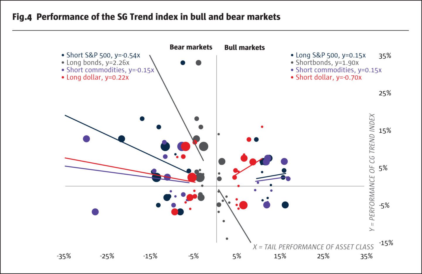
First, it’s possible to see that the SG Trend index benefits from either bull or bear regimes in all asset classes on average. We see a dispersion between the bear and bull periods: on average trend-followers benefit more in bear regimes than in bull regimes, which we illustrate in Figure 5. We can also see the dispersion in bull periods: bull regimes across different asset classes appear to be less clustered together than in bear regimes.
Second, we can observe an unexpected symmetry for bonds: while in the bear regime, a +5% gain in bonds is expected to contribute an +11% gain for the SG Trend index, in the bull regime, a -5% loss in bonds is expected to contribute a -9% loss for the SG Trend index. One possible explanation is that over the past two decades, bonds have been in a sustained bull market with occasional dips which trend-followers have not been able to capture. For commodities, we observe almost perfect symmetry: they are expected to contribute to trend-followers equally in bear and bull markets.
In Figure 4, we see an interesting asymmetry between bear and bull markets for both the amplitude of returns and the clustering of same regimes across asset classes. In bear markets, returns are larger in absolute terms and stresses tend to occur simultaneously in few asset classes. Do trend-followers benefit more from bear regimes than from bull regimes?
In Figure 5, we show the average quarterly return of the SG Trend index as a function of a number of bear and bull regimes across four asset classes (each quarter with more than two regimes is counted only once). We see that, on average, trend-followers benefit more in bear markets than in bull markets for two or three and four simultaneous crises in asset classes. This appears to be a new discovery. We call this effect the clustering skew of trend-following. Trend-followers cannot benefit from idiosyncratic bull or bear regimes in asset classes.
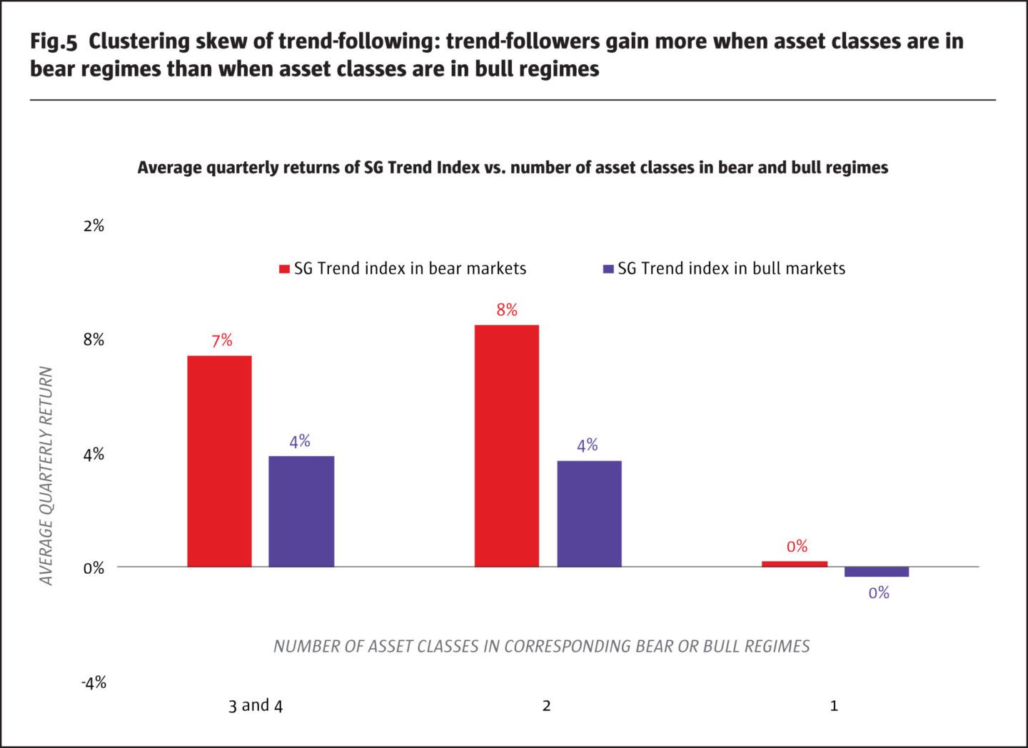
The clustering skew means that trend-followers are expected to benefit more from the clustering of bear regimes than from the clustering of bull regimes. For practitioners who are familiar with dispersion trading through options, the clustering skew of CTAs is analogous to the correlation skew in index options. On the one hand, we can be long the correlation skew through buying equity index options and selling options on stocks; on the other hand, we can be long the dispersion through buying options on stocks and selling index options. In a bear regime, index options will gain more than stock options creating a positive return. In a bull regime, the opposite effect takes place: stock options will gain more than index options because of the dispersion. In this comparison, trend-followers combine the best parts of the clustering/correlation and dispersion effects. Trend-followers are long clustering/correlation in bear markets and long the dispersion in bull markets. Bear markets are more beneficial for trend-followers due to returns on asset classes tending to be larger in magnitude and the clustering of bear regimes in asset classes.
Regime conditional model for the performance attribution
Since the performance of trend-following CTAs and other systematic ARP product can change significantly in different market regimes, how can we attribute risk-adjusted performance to varying market betas of these strategies? Importantly, after we account for the conditional beta exposures, is there any alpha in these strategies? We propose a regime-dependent regression model to explain and illustrate key differences between risk profiles of ARP products, hedge funds, and CTAs.
Our model is implemented as follows. First, we select a benchmark to analyse the performance of a strategy relative to this benchmark. In our examples, we choose the S&P 500 total return index. We specify the return frequency with non-overlapping periods (monthly, quarterly) and compute paired returns of the strategy and its benchmark. Then we sort the pairs by returns on the equity index. After the sorting, we label returns of the benchmark that are below the 16% quantile, which approximately corresponds to returns below one standard deviation, as belonging to the bear regime. In a symmetric way, we label returns above the 84% quantile, which correspond to returns above one standard deviation, as belonging to the bull market regime. Finally, we label returns in the middle (returns approximately within one standard deviation) as belonging to the normal regime. The empirical frequency of bear, normal, and bull regimes is 16%, 68%, and 16%, respectively.
Definition: the regime-conditional regression model
Strategy returns are regressed using return on the benchmark X by:
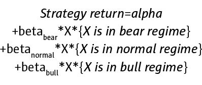
Here, X is the return of the benchmark and the bracket terms are the indicators for market regimes (only one condition will be true).
In statistics, this type of conditional regression is known as a segmented regression. We note that few researchers have proposed models with asymmetric betas, most notably a two regime model with betas for negative and positive index returns. However, we find that the explanatory power of such asymmetric beta models to be not as strong as in our model.
The important point here is that we keep the alpha constant across different regimes. On the one hand, empirically, regime conditional alphas turn out to be insignificant for most of products, unlike the regime conditional betas that are significant for most of them. On the other hand, we are interested in the overall alpha that a strategy can produce over the full life-cycle of equity markets including bull and bear regimes.
We can apply this model to analyse returns for different frequencies, such as weekly, monthly or quarterly by grouping returns to the 16%/84% quantiles (one standard deviation without any specific model assumption) and applying the grouping methodology as described above. Empirically, statistical quantiles scale across different frequencies, so that the model is applicable to different time horizons from daily to annual returns. For example, the quarterly quantiles scale to monthly quantiles as approximately the square root of 3, so the break-points of bear and bull regimes can be naturally compared to each other.
Illustrations for trend-following CTAs
By conditioning on market regimes, our model can detect the changing risk-profile of systematic strategies in these different regimes. For an example, does the pattern of real-world performance of trend-followers mimic the simplified trend-following strategy as described above? First, similarly to Figure 2, in Figure 6 we illustrate the scatter plot of returns of the SG Trend Index predicted by returns on the equity index at weekly and quarterly frequencies.
We observe that at weekly frequencies, the performance of the SG Trend Index follows a random pattern with respect to the equity index with insignificant betas. At quarterly frequencies, the SG Trend Index exhibits a significant negative beta to the performance of the equity index in the bear regime. Furthermore, trend-followers have higher equity betas in the normal and bull regimes, as equity markets tends to go up in the long-term.
The key message from our analysis is that trend-followers are more likely to deliver negative crisis betas during crises lasting over extended periods as most of trend-following CTAs apply medium- to long-time time horizons for signal generation. Consequently, trend-followers can serve as robust diversifiers of equity risk during corrections lasting over longer periods. In addition, returns of trend-followers should be measured at a relatively low frequency (at least quarterly) to analyse the diversification benefits.
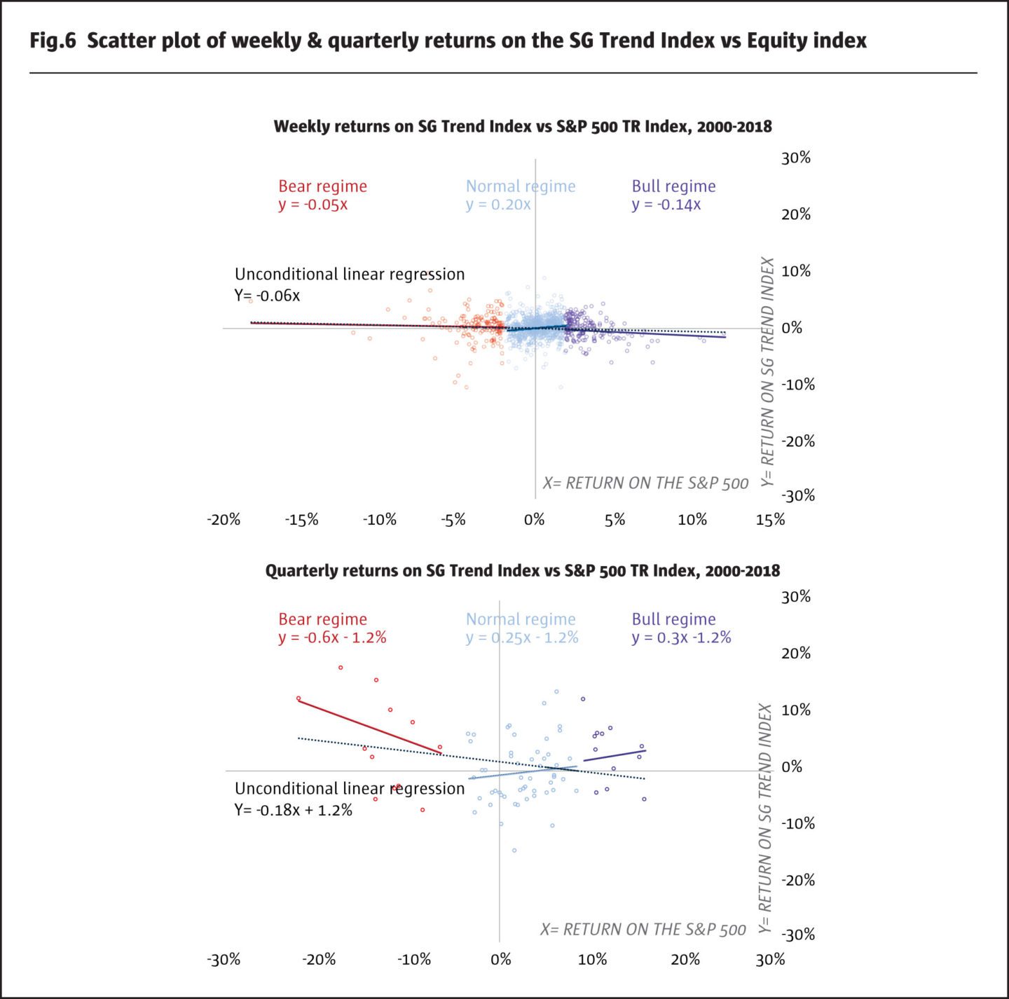
Importantly, we show a linear regression in Figure 6 to highlight the difference between the simple linear regression and our regime conditional regression. For quarterly returns, the linear regression indicates a negative bias of the SG Trend Index by overweighting large positive returns in the bear regime. Moreover, the linear model implies a small negative beta overall with positive alpha of 1.2% which is statistically significant. In contrast, the regime conditional regression implies negative overall alpha, which is however not statistically significant. Remarkably, the regime conditional illustrates how trend-following CTAs adjust to changing market regimes to generate either defensive or risk-seeking betas.
Trend-following CTAs: Crisis alpha or crisis beta?
When discussing the performance attribution of trend-following CTAs, some practitioners refer to crisis alpha as the outperformance of trend-following CTAs during equity crisis periods. However, as we show in Figures 3 and 4, trend-followers are expected to deliver significant performance only when the crises last over extended periods. As a result, most of the time, trend-following strategies cannot deliver diversification during short-lived corrections. Therefore, the question is whether the crisis performance of trend-following should be attributed to its actively managed negative, or crisis, beta to the equity market or to an idiosyncratic crisis-conditional alpha.
The analysis of the crisis performance is difficult because the very definition of a crisis period is rather arbitrary and different authors proposed various definitions. Also, it is not trivial to annualise and normalise the crisis performance in a meaningful way. In our illustration in Figure 3, the SG Trend index accumulated the total performance of 73% during the last two bear markets, where we define the crisis period to last in the first part of the drawdown in the equity market from peak to bottom. Should we include the period until the full recovery up to its high watermark, the perceived crisis alpha would decline because the SG trend index did not perform well during these times.
Definition of crisis alpha
To address the definition of a crisis for analysis of systematic strategies including trend-following CTAs, we apply a regime conditional regression model for ex-post returns as follows. The outputs are reported in Table 2.
1. We take the bear regime implied by our model to define the equity crisis. We recall that our model defines bear regimes as those quarters when the benchmark index declines by more than one standard deviation (16%-quantile).
2. We compute average quarterly returns on the S&P 500 index and SG Trend index and the quarterly risk-free rate using 3-month T-bill rate for each of the three regimes.
3. We calculate the regime-conditional returns by multiplying the average returns by the regime probability and by the annualisation factor (4 for quarterly returns).
4. We compute the regime conditional excess returns over the risk-free rate.
5. We take the regime-conditional betas, which are significant at 5%: only the conditional beta for the bear regime is significant. We compute the beta attribution from the S&P 500 index using the regime-conditional excess returns and significant betas.
6. We compute the beta-adjusted alpha of the SG Trend index as the difference between the regime-conditional excess return and the beta contribution.
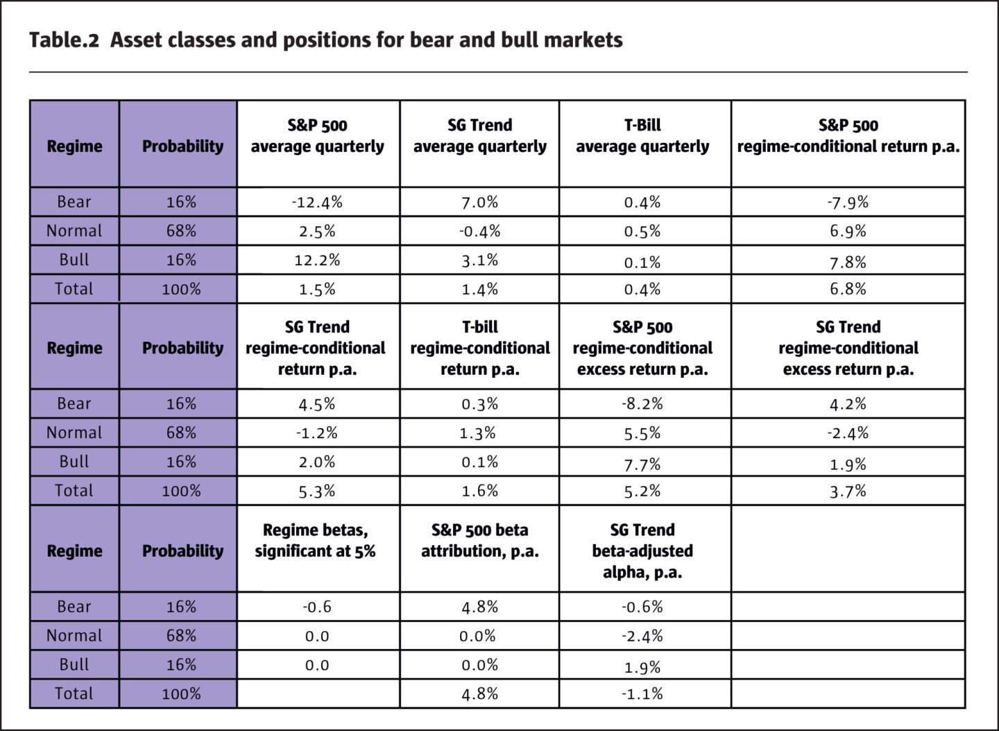
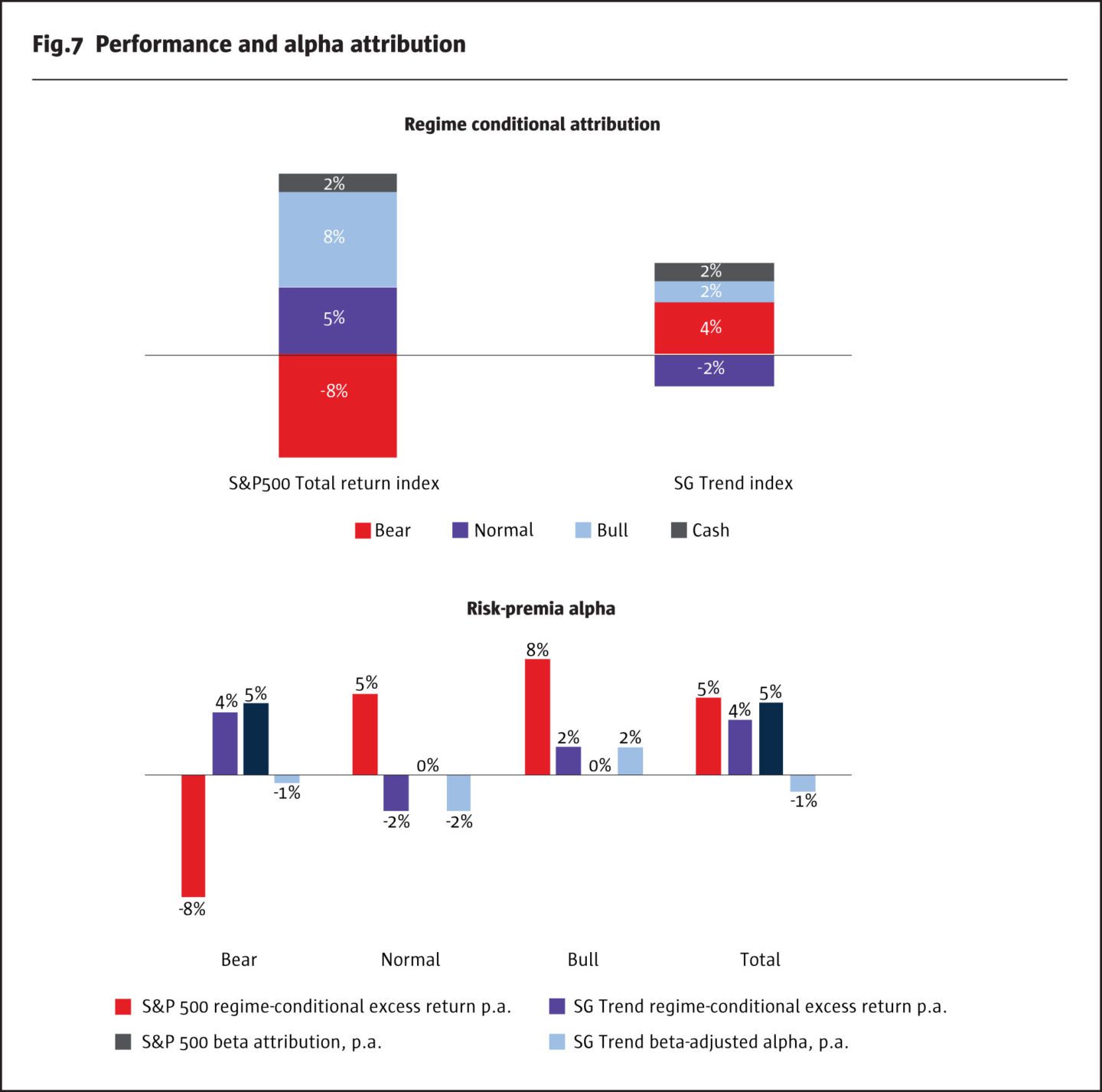
Our estimate is that 4.2% p.a. of the SG Trend index is attributed to crisis periods. This result is close to the estimate obtained by Kaminski of 4% p.a. in the influential white paper “In Search of Crisis Alpha”. In addition, we find that normal periods constitute the biggest drag at -2.4% p.a., which is only partially offset by 1.9% p.a. attributed to bull regimes.
Thus, our formal definition of a crisis is consistent with somewhat discretionary approaches and, importantly, we can apply our definition to analyse the crisis performance of CTAs conditional on other asset classes in a uniform way that can be easily reproduced by other researchers and practitioners. Therefore, we provide a formal definition.
Definition: Crisis alpha
The crisis alpha is the return on a systematic strategy attributed to the ex-post return in the bear regime. In our model, the crisis alpha is computed as:

Where the bear regime is defined by periods when returns on the benchmark are below the 16%-quantile of the empirical distribution of in-sample returns, average excess return is the average return on the strategy adjusted by the risk-free rate, and AF is the annualisation factor.
Defensive and risk-seeking strategies
While our definition defines the crisis alpha on average, we note that the excess return of the strategy in bear regime may be negative. However, over the long periods of time we can differentiate between:
1. Defensive strategies with positive crisis alpha
2. Risk-seeking strategies with negative crisis alpha
However, the crisis alpha alone cannot be used to characterise the long-term risk adjusted performance of systematic strategies. For an example, the systematic buying of index put options is a defensive strategy with a positive crisis alpha. However, over the long run, the excess return on this strategy is most likely to be negative because implied volatility of index put options is expensive. In addition, the strategy maintains a systematic short bias to the equity index because of systematically buying puts. Thus, we need to account for this bias for risk-adjusted attribution of strategy returns.
Definition of risk-premia alpha
We introduce the regime conditional alphas and risk-premia alpha to account for any systematic bias that a strategy may produce towards either short or long exposures to its benchmark in a statistically significant way.
Definition: beta-adjusted bear alpha and the risk-premia alpha
The beta-adjusted bear alpha is the return on a systematic strategy after attribution to the beta exposure computed by:
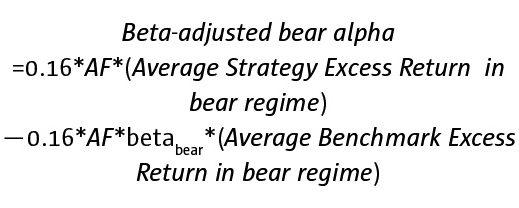
where the bear regime is defined as before and betabear is the bear beta which is an estimate from the regime conditional regression model. We use the estimate of the bear beta only if it significant at the 5% level, otherwise we assume the bear beta to be zero.
In the same way, we compute beta-adjusted alphas for the normal and bull regimes. We define the risk-premia alpha as the sum of beta-adjusted regime alphas.
We argue that the risk-premia alpha provides the proper way to analyse the risk-adjusted returns on systematic strategies, which may have changing risk profile in different market regimes. Our definition of risk-premia alpha can be interpreted as Jensen’s alpha in a regime conditional CAPM. In an empirical analysis, we show that there is a strong empirical link between risk-premia alphas and bear betas.
Table 2 and the right side of Figure 7 report the beta-adjusted alpha for the SG Trend index. The index produces a small negative beta-adjusted alpha which cannot be explained by the performance of the equity market in bear regime. We see that the SG Trend Index produces insignificant alpha in all regimes, with the total alpha of about -1% p.a.
To summarise, the performance of the SG Trend Index in the bear regime can be solely attributed to its significant negative index beta. Thus, positive returns that trend-followers may produce in bear regimes may be attributable to actively managed market betas, or market timing, rather than crisis alpha or beta-adjusted risk-premia alpha. We argue that it is a special skill provided by trend-followers to deliver equity market betas that change conditional on market regimes without compromising too much of the long-term alpha. As a result, trend-following CTAs are a niche asset class that well deserve a place in traditional and alternative portfolios.
Risk-premia alpha as compensation for the tail risk
In the past few years, we have experienced an influx of alternative risk-premia products from the sell side as a cheap replication of hedge funds, including trend-following CTAs. However, 2018 proved to be a very difficult year for most ARP products and, in parallel, for trend-following CTAs. Nevertheless, we emphasise that ARP products and trend-following have different risk profiles and different sources of their performance in the long run.
To quantify changes in the risk profile of a systematic strategy in bear and bull regimes, we again apply our regime conditional regression model which we present in terms of marginal bear and bull.
Definition: the regime-conditional regression model with marginal bear and bull betas
Strategy returns are regressed using return on the benchmark X by:
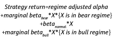
Statistically, using the least squares estimation, this model is equivalent to the regime conditional model introduced before and, in particular, the following identities hold:

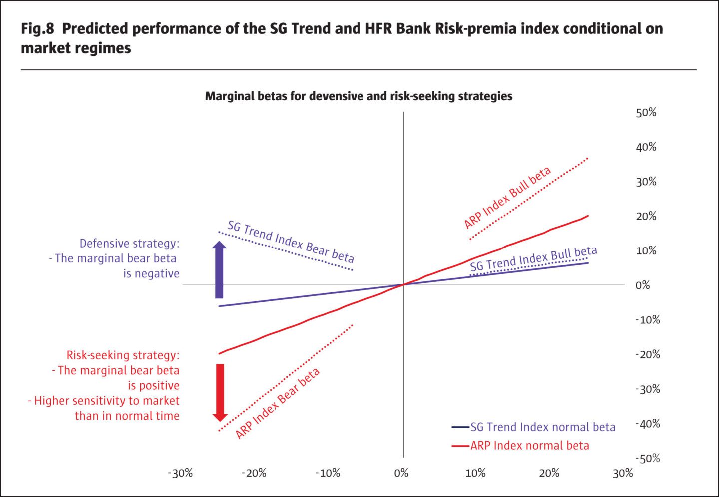
In Figure 8, we illustrate the regime-dependent regression model for the flagship Bank Multi-Asset Risk-premia Index using the performance of the S&P 500 index. The model produces a high explanatory power of 65% for the ARP index and about 20% for the SG Trend index. Our model implies that the ARP index is leveraged to the downside and to the upside. In contrast, the SG Trend index has a small beta in the normal regime but its beta changes to negative in bear regime.
The marginal beta indicates how significantly the risk profile of a systematic strategy can change when the market transitions to either bear or bull market regimes. The defensive strategy will have a negative marginal beta in the bear regime indicating that the performance of the strategy has smaller sensitivity in the bear regime or, if the total beta becomes negative, the strategy benefits from negative performance of the index.
Risk-premia alphas for CBOE volatility indices
More often than not, systematic ARP strategies and hedge funds have positive marginal bear betas. Do they earn excess alpha? Following the CAPM, returns on an asset must be seen as a compensation to take the beta risk. However, empirically it is well established the market beta is a poor indicator of the risk-adjusted performance and the risk profile of any asset. As evidence, many risk-seeking strategies, including short volatility strategies that sell tail risk protection, tend to have insignificant market betas during normal regimes but their betas may explode in bear regimes. Using our regime conditional model, we propose that the marginal bear beta serves as a measure of the tail risk of an asset and that the regime adjusted alpha serves as a measure of the risk-premia that the asset must earn to compensate for its marginal bear beta.
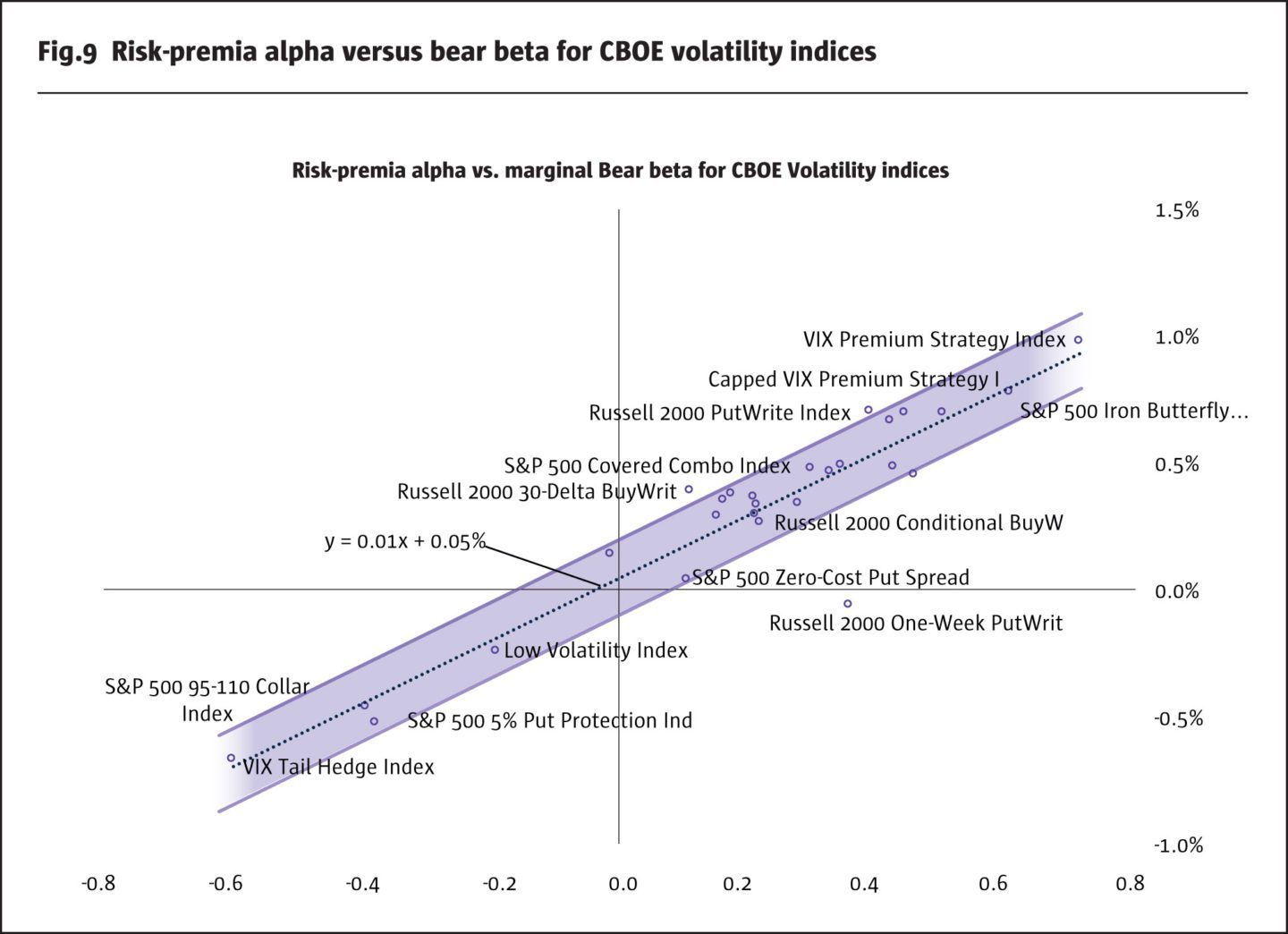
In our first cross-sectional study, we consider CBOE volatility benchmark indices, which systematically sell or buy index options on the S&P 500 index with various degrees of risk. The volatility benchmark indices are particularly good for our study because of their asymmetric tail risk inherent to all short volatility strategies. Also, it is well-known that these strategies may earn in the long-term as a risk-premia compensation. CBOE publishes time series of 28 benchmark indices with the time series for most of them going back to 1987, so that the sample includes all crises of the past three decades. In Figure 9, we first plot the risk-premia alpha versus the marginal bear betas and then we estimate the regression line connecting these pairs.
We see that our regime conditional model is strongly supported by the data. The larger the marginal beta, the higher the risk-premia alpha the strategy produces. In reverse, the risk-premia alpha is negative for defensive strategies which buy index puts to limit the downside exposure. Finally, in line with intuition, if a strategy does not take any marginal risk, it is not expected to produce any risk-premia alpha because the intercept of the regression line is close to zero.
To conclude, the marginal bear betas serve as a measure for risk-premia. As comparison to other studies, we mention CFM’s research paper “Risk premia: asymmetric tail risks and excess returns”. CFM’s researchers argue that the excess performance on the risk-premia strategies is derived from the skewness of their returns. Consequently, assets and strategies with large negative skew require a compensation to suffer steep losses asymmetric to potential gains. Empirically, we found that skewness alone cannot explain the excess returns and alpha on ARP strategies including CBOE volatility indices and hedge funds. As a result, our model takes an extra step by assuming that the risk-premia alpha should be attributed as a compensation for suffering steep losses in bear regimes, not only as a compensation to asymmetric losses overall.
Trend-following CTAs vs ARP products
One of the most typical questions is how alternative risk-premia products are different from hedge fund products, in particular, from CTAs? To illustrate different risk profiles of hedge fund and ARP products, we apply the regime conditional model to a large universe of indices grouped into three categories:
1. Hedge fund indices from major index providers including HFR, SG, BarclayHedge, Eurekahedge with the total of 73 composite hedge fund indices excluding CTA indices;
2. 7 CTA indices from the above providers; and
3. ARP indices using HFR Bank Systematic Risk-premia Indices with a total of 38 indices.
First, we estimate the regime conditional regression model for the whole universe using the S&P 500 total return index as the benchmark. For each index, we use the time series from its inception up to year-end of 2018. Then, we take the indices for which the regression has significant explanatory power R2 of at least 5% yielding a sample of about 80% of the whole universe. Finally, we apply cross-sectional regressions to each category to explain risk-premia alphas using marginal bear betas.
In Figure 10, we illustrate the relationship between risk-premia alphas and marginal bear betas. Our cross-sectional regression explains about 35% of the cross-sectional data. Similarly to CBOE volatility indices, we observe a strong linear relationship between risk-premia alphas and marginal bear betas for hedge fund and ARP indices. Consequently, part of the performance of ARP products and hedge funds can be attributed to exposures to the tail risk.
Interestingly, we see that the positive slopes, which indicate how much risk-premia alpha is produced by increasing marginal bear beta, are very similar for hedge fund and ARP indices. This evidence indicates that there is a linear relationship between the exposure to tail risk and the required compensation across different risk-premia strategies. However, the intercept of the regression line for the hedge fund indices is positive while the intercept for ARP indices is significantly negative. As a result, ARP products are expected to provide less efficient risk-premia alpha. In other words, a risk-seeking investor, who looks for risk-premia products as a compensation to take the tail risk, is better off to stick with traditional hedge fund products.
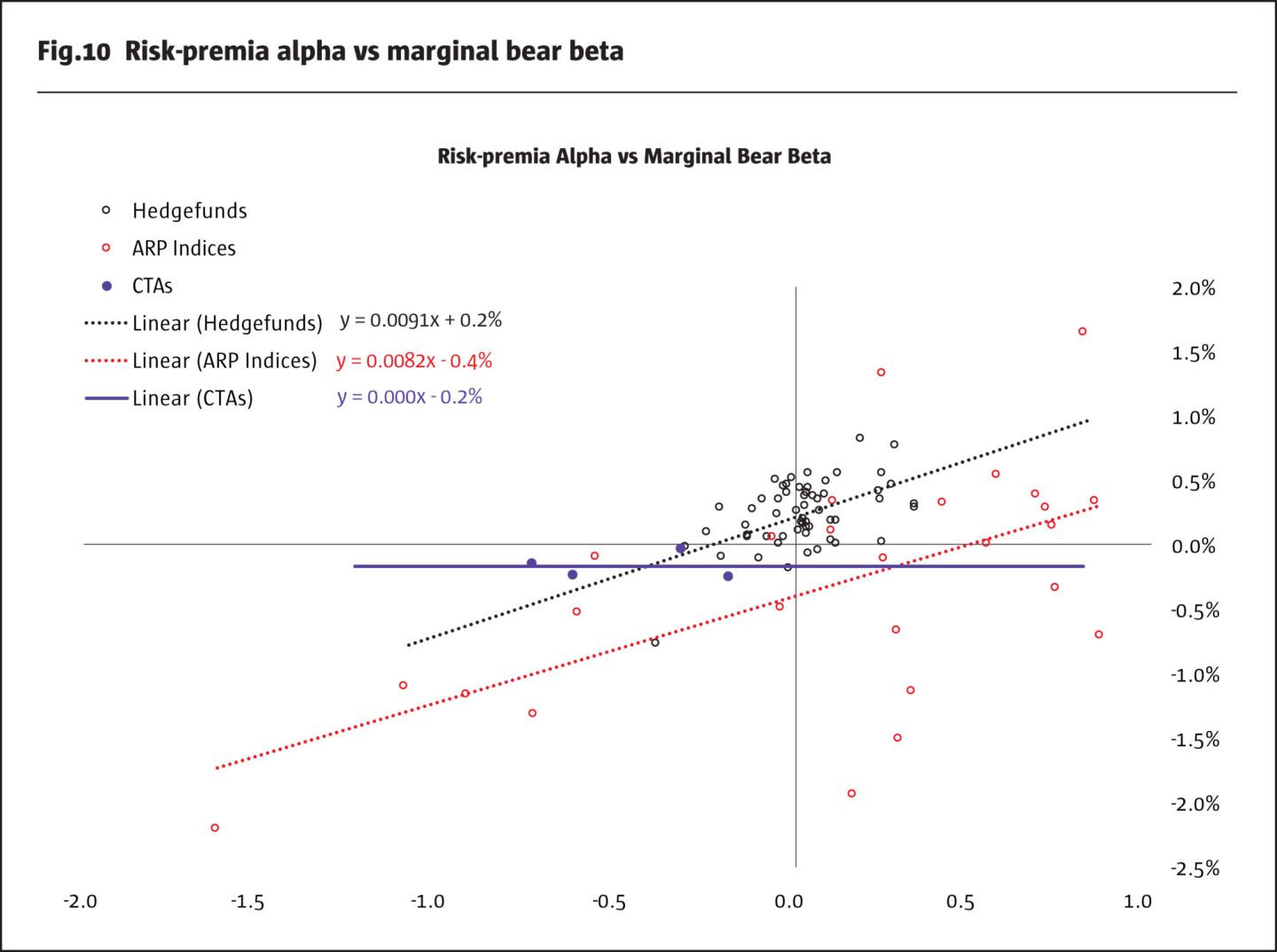
Finally, we find that CTAs stand out as exceptions because they produce defensive bear betas with small negative risk-premia alpha, which is about the same across the four CTAs indices in our final sample. This implies that CTAs should be viewed as defensive, actively-managed strategies that are expected to deliver positive performance in bear markets with flat to negative risk-premia alphas.
CTAs in portfolios of ARP and hedge fund products
We have shown that CTAs produce defensive equity betas in bear markets with insignificant risk-premia alphas. In contrast, most hedge fund and ARP products produce positive risk-premia alphas as compensation for positive marginal bear betas. CTAs and trend-following CTAs may serve as diversifiers for a portfolio of alternatives. By mixing CTAs with ARP and traditional hedge fund products, investors and allocators can achieve improved risk-reward profiles in terms of both portfolio volatility and tail risk exposure.
In Figure 11, we illustrate risk-reward profiles of portfolios produced by mixing the SG Trend Index and the HFR Bank Systematic Risk Premia Multi Asset Index. We compute portfolio returns, volatility and bear betas ex-post from 2007 to end of 2018. We observe that by varying the weights of CTAs, we can achieve different risk-profiles of alternatives portfolios.
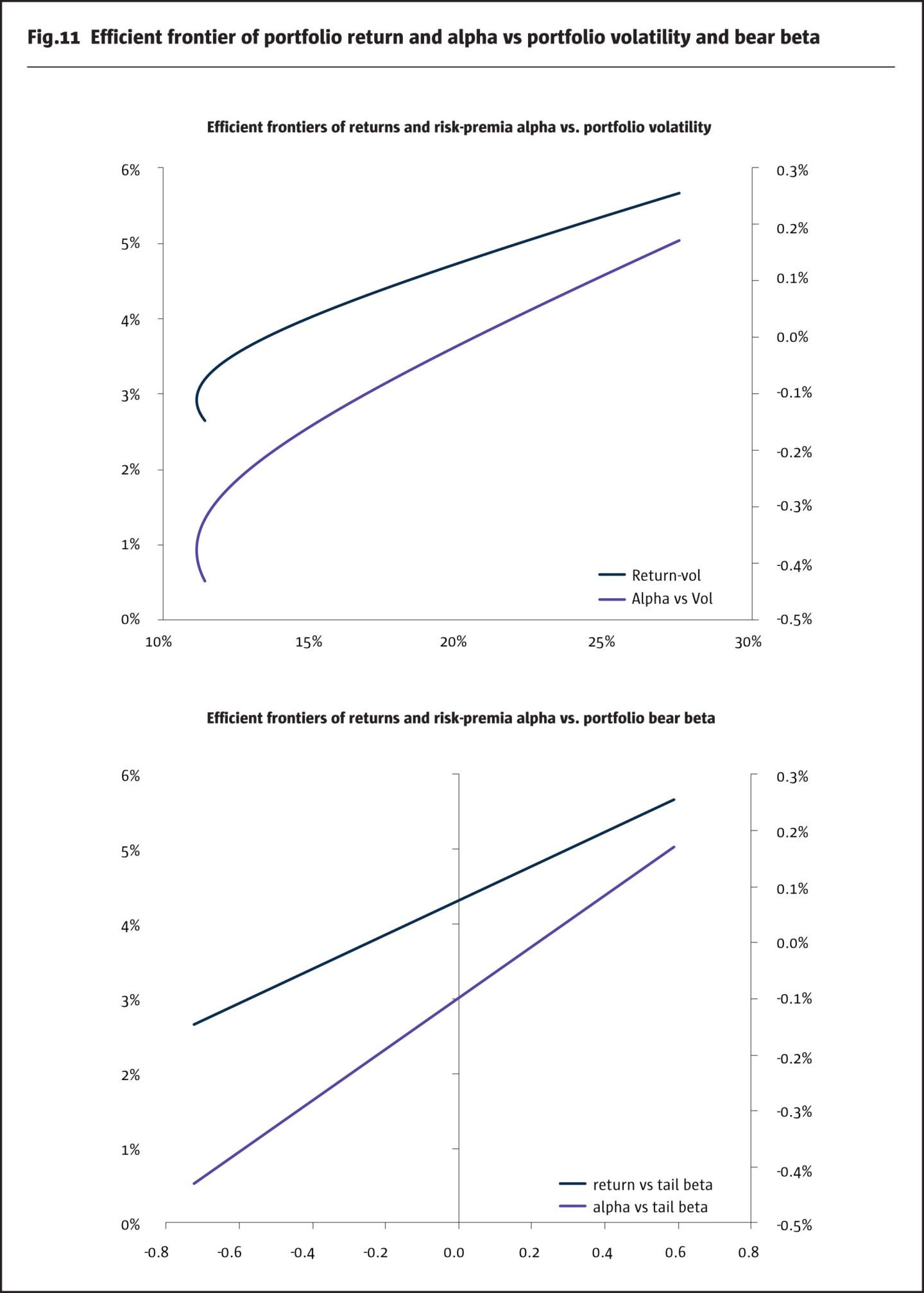
When portfolios are analysed in terms of portfolio volatility, there is an optimal portfolio achieving the minimum portfolio volatility and the risk-reward frontier is concave. However, when portfolios are viewed in terms of marginal bear betas, the risk-reward frontier is linear. The key conclusion for investors and allocators is that alternatives portfolios must be viewed as a trade-off between the expected risk-premia alpha and bear betas. This trade-off must be matched by the risk profile of each investor. Our regime conditional model can serve as a tool to analyse this trade-off at the portfolio level.
End Notes
Data Source: Quantica Capital AG, Bloomberg
Fig.1 & 2
S&P 500 TR Index – SPTR
Data from 02/09/2008 – 20/11/2008
Fig.3
SG Trend Index – NEIXCTAT
S&P 500 TR Index – SPTR
Data from 01/01/2000 – 31/12/2018
Fig.4&5
SG Trend Index – NEIXCTAT
S&P 500 TR Index – SPTR
U.S. dollar Index – DXY
Barclays US Agg Total Return Value – LBUSTRUU
Bloomberg Commodity Index – BCOM
Data from 01/01/2000 – 31/12/2018
Fig.6&7
S&P 500 TR Index – SPTR
SG Trend Index – NEIXCTAT
Data from 01/01/2000 – 31/12/2018
Fig.8
S&P 500 TR Index – SPTR
HFR Bank Systematic Risk Premia Index – HFRRMA
SG Trend Index – NEIXCTAT
Data from 01/01/2000 – 31/12/201
Fig.9
CBOE Volatility indices – http://www.cboe.com/products/strategy-benchmark-indexes
HFR Bank Systematic Risk Premia Index – HFRRMA
Data from products inception – 31/12/2018
Fig.10
Hedge Funds: HFR, BarclayHedge, Eurekahedge hedge funds universe|
CTAs: HFRXM Index, HFRXSDV Index, NEIXCTAT Index, NEIXSTTI Index
ARP: HFR ARP universe
Data from products inception – 31/12/2018
Fig.11
SG Trend Index – NEIXCTAT|HFR Bank Systematic Risk Premia Index – HFRRMA
Data from 31/07/2007 – 31/12/2018
S&P 500 TR Index – SPTR
Data from 02/09/2008 – 20/11/2008
SG Trend Index – NEIXCTAT
S&P 500 TR Index – SPTR
Data from 01/01/2000 – 31/12/2018
SG Trend Index – NEIXCTAT
S&P 500 TR Index – SPTR
U.S. dollar Index – DXY
Barclays US Agg Total Return Value – LBUSTRUU
Bloomberg Commodity Index – BCOM
Data from 01/01/2000 – 31/12/2018
S&P 500 TR Index – SPTR
SG Trend Index – NEIXCTAT
Data from 01/01/2000 – 31/12/2018
S&P 500 TR Index – SPTR
HFR Bank Systematic Risk Premia Index – HFRRMA
SG Trend Index – NEIXCTAT
Data from 01/01/2000 – 31/12/201
CBOE Volatility indices – http://www.cboe.com/products/strategy-benchmark-indexes
HFR Bank Systematic Risk Premia Index – HFRRMA
Data from products inception – 31/12/2018
Hedge Funds: HFR, BarclayHedge, Eurekahedge hedge funds universe|
CTAs: HFRXM Index, HFRXSDV Index, NEIXCTAT Index, NEIXSTTI Index
ARP: HFR ARP universe
Data from products inception – 31/12/2018
SG Trend Index – NEIXCTAT|HFR Bank Systematic Risk Premia Index – HFRRMA
Data from 31/07/2007 – 31/12/2018
Biographies
Artur Sepp
Director of Research at Quantica Capital AG in Zurich. Artur focuses on systematic data-driven trading strategies. Artur has taken several leading roles as a quantitative strategist since 2006. Prior to joining Quantica, Artur worked at Julius Baer in Zurich, developing algorithmic solutions and strategies for the wealth management and portfolio advisory. Prior to this, Artur worked as a front office quant strategist for equity and credit derivatives trading at Bank of America Merrill Lynch in London and Merrill Lynch in New York. Artur has a PhD in Statistics, an MSc in Industrial Engineering from Northwestern University, and a BA in Mathematical Economics. His primary expertise is in econometric data analysis, machine learning, and computational methods along with their applications for quantitative trading strategies and asset allocation. He is the author and co-author of several articles on quantitative finance published in leading journals. He is also known for his contributions to stochastic volatility and credit risk modelling.
Louis Dézeraud
Senior Marketing and Client Relationships at Quantica Capital AG. Before joining Quantica, Louis worked in the Investor Relations team at Jabre Capital Partners. Prior to that, he supported the Business Development Unit’s growth of Natixis Global Asset Management in Amsterdam. Louis started his career at Olympia Capital Management in Paris.
Director of Research at Quantica Capital AG in Zurich. Artur focuses on systematic data-driven trading strategies. Artur has taken several leading roles as a quantitative strategist since 2006. Prior to joining Quantica, Artur worked at Julius Baer in Zurich, developing algorithmic solutions and strategies for the wealth management and portfolio advisory. Prior to this, Artur worked as a front office quant strategist for equity and credit derivatives trading at Bank of America Merrill Lynch in London and Merrill Lynch in New York. Artur has a PhD in Statistics, an MSc in Industrial Engineering from Northwestern University, and a BA in Mathematical Economics. His primary expertise is in econometric data analysis, machine learning, and computational methods along with their applications for quantitative trading strategies and asset allocation. He is the author and co-author of several articles on quantitative finance published in leading journals. He is also known for his contributions to stochastic volatility and credit risk modelling.
Senior Marketing and Client Relationships at Quantica Capital AG. Before joining Quantica, Louis worked in the Investor Relations team at Jabre Capital Partners. Prior to that, he supported the Business Development Unit’s growth of Natixis Global Asset Management in Amsterdam. Louis started his career at Olympia Capital Management in Paris.
- Explore Categories
- Commentary
- Event
- Manager Writes
- Opinion
- Profile
- Research
- Sponsored Statement
- Technical